2. DBMS Systems

This is the DBMS Systems course theme.
[Complete set of notes PDF 625Kb]

2.1. Queries

In this lecture we look at...
[Section notes PDF 319Kb]

2.1.01 Introduction

  • Methods of getting data out
  • The need for queries
  • QBE
  • SQL (design side)
    • History
    • Schemas and relations (CREATE)
    • Data types and domains
    • DROP and ALTER

2.1.02. Querying interfaces

  • High (view) level
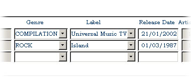
  • Query-By-Example (QBE)
    • Alternative to SQL
      • Table driven (visually similar to relations)
      • Rather than script driven, hence intuitive over learned
      • Visual or text based
    • User fills in templates
    • Microsoft Access approach

    Query-by-example from MS Access

2.1.02b. QBE visual example

  • Record advancing
  • Query designing
    • Finite domain attributes
    • Web search parallel

Record manoeuvring in Visual QBE (Access)Query definition in Visual QBE (Access)

2.1.03. QBE text-format example

  • P. print, I. insert, D. delete, U. update
  • _VARNAME, copy field value into variable

Query by example (Text)

2.1.05. SQL

  • Structured Query Language
  • Success of relational databases
  • Developed for SystemR at IBM
  • ANSI standardised
  • SQL-1986 (SQL1), ongoing extension
  • SQL-1992 (SQL2), current version (Oracle 9i)
  • SQL-1999 (SQL3), regular expression matching, recursive queries
  • SQL-2003, XML features, auto-generated columns

2.1.05b. SQL command syntax

  • Where follows here is a brief summary
    • Oracle syntax
    • Similar but not identical to MySQL/MSSQL
  • General familiarity
  • Query writing best learnt by doing it
  • Lecture live-example
  • Coursework 1 will be SQL
  • Oracle (9i) SQL reference
  • MySQL (5.0) SQL reference

2.1.05c. SQL in application

  • Keyword oriented language
  • Keywords not congruous with Relational model
  • Lots of different ways to write SQL
    • Analogous to C/Java formatting
    • if (b==2) { a=1; } else { a=0; }
  • Recommend using case to differentiate attributes and keywords
    • SELECT colour, size, shape FROM fruit WHERE weight>22;
  • Oracle user accounts on Teaching database
  • Namespace references, e.g. shared.cars

2.1.06. SQL Create schema

  • Data definition commands
  • CREATE
    • SCHEMA <schema_name> AUTHORIZATION <a>
    • or workspace
  • Beware of names
    • Name collisions produce odd behaviours
  • SQL Schema embraces Tables (relations), constraints, views, domains, authorizations

2.1.07. SQL Create table

  • CREATE TABLE
    • <schema_name>.<relation_name>
    • (
      • <attribute_definitions>
      • <key>
      • <constraints>
    • )
  • CREATE TABLE example (Oracle)
  • Tables can (and should) be indexed by user
  • e.g. <username>.<tablename>
  • Normal login implies username
  • Non-local table access

2.1.08. Data types and domains (Oracle)

  • Numeric
    • ENUM
    • NUMBER, NUMBER(i), NUMBER(i,j)
      • Formatted numbers, i precision, j scale
      • (number of digits total, after decimal point)
    • Character-string
      • CHAR(n) - n is length
      • VARCHAR2(n) - n is max
    • DESCRIBE output example
    • Multi-database comparison of Datatypes
    • Database legacy: limited storage necessitated efficient storage
    • Does it need to be efficient anymore?

    You might consider all SQL types as being conceptually similar to attribute types in the relational model, although in reality the implementation of these types in a DBMS only approximates the mathematical purity of unordered domain sets etc.

2.1.08b. Data types and domains (MySQL)

  • Numeric
    • TINYINT, INT, INT UNSIGNED
    • FLOAT, DOUBLE, DECIMAL
    • ENUM
    • Character-string
      • CHAR(n) - n is length
      • VARCHAR(n) - n is max
      • TINYTEXT, TEXT
      • Beware different default/maximum lengths to Oracle
    • BLOB
    • Multi-database comparison of Datatypes

2.1.09. Time-based data types

  • Date and Time
    • DATE
      • Ten positions, components YYYY-MM-DD
    • TIME
      • Eight positions, components HH:MM:SS
    • TIME(i)
      • Time fractional seconds precision
      • Adds i+1 positions
    • TIMESTAMP
      • optionally WITH TIME ZONE
    • Very sensitive to syntactical ambiguities
      • day/month/year/hour/minute separators

2.1.10. DROPing

  • DROP <object> <obj_name> <flags>
  • DROP SCHEMA <schema_name> CASCADE
    • drops all workspace tables, domains
  • DROP TABLE <relation_name> RESTRICT
    • only drops table if
    • not referenced in any constraints/views
  • Notion of cascading
  • Table links

2.1.11. ALTERing

  • Schema evolution
  • Design side
  • ALTER TABLE <schema_name>.<relation_name> ADD
    <var_name> <var_type>;
  • Example
    • ALTER TABLE uni.student ADD hall VARCHAR(32);
  • Upper and lower case syntax
  • Naming conventions

2.1.12. Queries

  • Helper interfaces
    • HeidiSQL/phpMyAdmin/Sword/SQLplus
    • Design/perform a lot of routine queries for you
    • Important to learn SQL, reinforcement
    • Designing select queries is more difficult
    • Visual interfaces still lacking in this area
  • Select queries in SQL
  • Basic singlets
  • Renaming
  • Queries with Joins
  • Nested queries

2.1.13. SQL Queries

  • SELECT statement
  • Similar to relational data model SELECT then PROJECT
    • SELECT <attribute list>
    • FROM <table list>
    • WHERE <condition>;

Select query cropping example

2.1.14. SQL Queries

  • SELECT <attr_list>
    • FROM R,S,T
    • WHERE DNO = 10
  • equivalent to
  • p<attr_list>(sDNO=10 (R X S X T))
  • True-false evaluation tuple by tuple
  • WHERE clause as compound logical statement

2.1.15. SQL Queries

  • Produces a relation/set of tuples
  • Can be used to extract a single tuple
  • e.g. SELECT bday, age
    • FROM student
    • WHERE fname='Tim' AND lname='Smith'
    • Result = (13-05-80, 20)
  • Argument quoting (')
    • SQL poisoning
    • Not null
    • Not numeric values
  • MySQL Attribute quoting (`)
    • Hypothetical attribute `all`, all, and ALL

SQL poisoning is a vulnerability exposed by inadequate escaping of arguments/variables used to compose SQL queries.

E.g. Tim in previous example, could be Tim'; DELETE FROM student;' SELECT * FROM student WHERE 1

2.1.16. Renaming and referencing

  • AS keyword
  • (Partial) Attribute renaming in projection list
    • SELECT fname AS firstName, minit, lname AS surname...
  • Role names for relations
    • SELECT S.FNAME, F.FNAME, S.LNAME
      • FROM STUDENT AS S, STUDENT AS F
      • WHERE S.LNAME=F.LNAME
  • (Total) Attribute renaming in FROM
    • SELECT s.firstName, s.surname
      • FROM student AS s(firstName,surname,DOB,NINO,tutor)
  • Wildcards (SELECT s.* FROM...)

2.1.17. SQL Tables

  • Relations are bags, not sets
    • e.g. projection of non-key attributes
  • Set cannot contain duplicate item/repetition
  • Duplicates exist in bags and be:
    • SELECT DISTINCT (eliminated)
    • SELECT ALL (ignored/kept)


2.1.18. Queries and Joins

  • Relational database allows inter-related data
  • SQL select FROM gives Cartesian product
  • WHERE clause defines join condition
    • SELECT proj.pnum, mgr.ssn
    • FROM project AS proj, employee AS mgr
    • WHERE proj.mgrssn = mgr.ssn;
  • Alternatively, explicitly define join (note type)
    • SELECT project.pnum, employee.ssn
    • FROM project INNER JOIN employee
    • ON project.mgrssn = employee.ssn;

2.1.18b. Outer joins

  • Outer joins are crucial in the real-world
  • Databases often contain NULLs (3VL)
  • Analysis of where the crucial data is across a relationship
  • Previous example, only get project data for managed projects
    • SELECT project.*, employee.*
    • FROM project INNER JOIN employee
    • ON project.mgrssn = employee.ssn;

Inner join example

2.1.18c. Outer joins (cont)

  • Scale of loss isn't always instantly obvious
  • NULLs often used unpredicably
  • May want project information, even if no employee attached as manager
    • SELECT project.*, employee.*
    • FROM project LEFT OUTER JOIN employee
    • ON project.mgrssn = employee.ssn;

    Outer join example

    2.1.19. 2y and 3y joins

    • Queries can encapsulate any number of relations
      • Even one relation many times (in different roles)
    • Relationship chain
    • Across many relations
      • Tuples as Entities OR Relationships
    • e.g. Employee -> Works_on -> Project -> Department ->
      Manager

    2.1.20. Recursive closure

    • Can’t be done in SQL2
    • Recursive relationships
    • Unknown number of steps
    • SQL2 can’t generalise in single query

    2.1.21. Nested queries

    • Essential one or more (inner) queries within an (outer) query
    • Inner and outer query
    • Not to be confused with inner and outer joins
    • Inner query can go in three places
      • SELECT clause (projection list)
        • Must return a single value, then aliased as attribute in outer result
      • FROM clause
        • Inner query result used as standard table in FROM cross product
      • WHERE clause

    2.1.21b. Nested query example

    • Use of query result as comparator for other (outer) query
      • SELECT DISTINCT course
      • FROM dept WHERE course IN (
        • SELECT d.course
        • FROM dept AS d, faculty AS f, student AS s
        • WHERE d.ownfac=f.id AND s.owndept=d.id
        • AND f.name='Eng' AND s.year='3'
      • ) OR course IN (
        • SELECT course
        • FROM dept
        • WHERE code LIKE 'COMS3%');

    2.1.22. Bridging SQL across 3 tiers

    • Three tier database design
    • Changing role of DBMS
    • Indices
    • Aggregate functions (conceptual)
      • Over bags and sub-bags
    • Creating and updating views (ext)
    • SQL embedding

    Three tier database design (Internal, Conceptual, External)

    In this subsection we look at the different roles SQL play across the three tiers of database design. We discuss the areas in which SQL is lacking and how those difficiencies can be complemented by embedding SQL in other languages.

    2.1.25. Indices

    • Low/Internal level
    • Index by one attribute
    • For queries selecting by that attribute:
      • Faster tuple access (ordered tuples)
      • Reduces database memory load
        • Small cross product relation, only crosses requisites
      • Accelerates query resolution time
    • CREATE INDEX Index_Name ON RELATION(Attribute);

    2.1.26. Aggregate functions

    • Run over groups of tuples
    • Takes a projected attribute list as an argument
    • Produce relation with single tuple
    • SUM, MAX, MIN, AVG, COUNT
    • e.g. AggFunc over all tuples
      • SELECT SUM(SALARY), MAX(SALARY), MIN(SALARY)
      • FROM EMPLOYEE;
    • Single attribute lists (distinct values)
    • Multi-attribute lists (granularity of distinct values by pairing)

    2.1.27. Aggregates over sub-bags

    • Can run over subsets of tuples
    • GROUP BY keyword
    • Specifies the grouping attributes
    • Need to also appear in projected attr_list
    • Show result along side value for group attr
    • e.g. AggFunc over subgroups
      • SELECT dno, COUNT(*)
      • FROM employee
      • GROUP BY dno

    Quick SQL check, do all attributes in the SELECT projection list appear in the GROUP BY projection list.

    2.1.28. Creating views

    • Views are partial projections
    • Virtual relations, or views of live relations
    • Update synchronised
      • CREATE VIEW <virtual_relname>
      • AS <real_relation>
    • Real relation could be a query result
    • Clever bit is the change propagation
    • UPDATEs made to the view dataset are flooded back to relations
      • INSERT and DELETE behaviour needs to be defined
      • Non-trivial as INSERT into view (virtual relation) may leave holes in real relation

    2.1.29. Embedding SQL

    • SQL (alone) can do lots of clever things in one expression
    • But can only execute a single expression
    • Can structure SQL commands into proper programming languages
    • Java Database Connection (JDBC)
      • javac, then java VM
    • COBOL, C or PASCAL
      • precompiled with PRO*COBOL or PRO*C
    • Procedure Language (PL/SQL)
      • Oracle/MySQL procedural language
      • Stored procedures can take parameters

    2.2. Internals

    In this lecture we look at...
    [Section notes PDF 180Kb]

    2.2.01. Introduction

    • Database internals (base tier)
    • RAID technology
      • Reliability and performance improvement
    • Record and field basics
    • Headers to hashing
    • Index structures

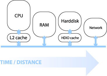
    2.2.01b. Machine architecture (by distance)

    • Distance from chip determines minimum latency
    • Speed of light is a constant
    • Impact of bus frequencies
      • IDE (66,100,133 Hz)
      • PCI, PCI-X (66,100,133 Hz)
      • PCI Express (1Ghz to 12Ghz)
    • Impact of bus bandwidths
      • PCI (32/64 bit/cycle, 133MB/s)
      • PCI Express (x16 8.0GB/s)

    Computer components by distance from processor

    Here's a link from Intel showing a machine architecture with signal bandwidths: Intel diagram

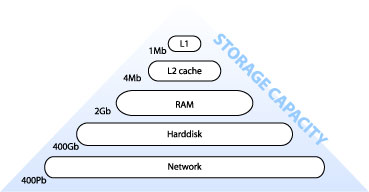
    2.2.01c. Machine architecture (by capacity)

    • Capacity increased with distance
    • Staged architecture as compromise
    • Speed, time/distance
    • Also cost, heat, usage scale

    Computer components by capacity

    2.2.02. Database internals

    • Stored as files of records (of data values)
      • Auxiliary data structures/indices
    • 1y and 2y storage
      • memory hierarchy (pyramid diagram)
      • volatility
    • Online and offline devices
    • Primary file organisation, records on disk
      • Heap - unordered
      • Sorted - ordered, sequential by sort key
      • Hashed - ordered by hash key
      • B-trees - more complex

    2.2.03. Disk fundamentals

    • DBMS task
      • linked to backup
    • 1y, 2y and 3y
      • e.g. DLT tape
    • Changing face of current technology
      • Impact of inexpensive harddisks
      • Flash memory devices (CF, USB)
    • Random versus sequential access
    • Latency (rotational delay) and
    • Bandwidth (data transfer rate)

    2.2.04. RAID technology

    • Redundant Array of Independent Disks
    • Data striping
      • Blocks (512 bytes), bits and transparency
    • Reliability (1/n)
      • Mirroring/shadowing
      • Error correction codes/parity
    • Performance (n)
      • Mirroring (2x read access)
      • Multiple parallel access

    2.2.05. RAID levels

    • 0 No redundant data
    • 1 Disk mirrors (performance gain)
    • 2 Hamming codes (also detect)
    • 3 Single parity disk
    • 4 Block level striping
    • 5 and parity/data distribution
    • 6 Reed-Soloman codes

    2.2.06. Records and fields

    • DBMS specific, generally
    • Records (tuples) comprise fields (attributes)
    • File is a sequence of records
    • Variable length records
      • Variable length fields
      • Multi-valued attributes/repeating fields
      • Optional fields
      • Mixed file of different record types

    2.2.07. Fields

    • records -> files -> disks
    • Fixed length for efficient access
    • Networking issues
    • Delimit variable length fields (max)
    • Explicit record/field lengths
    • Separators (,;,:,$,?,%)
    • Record headers and footers
    • Spanning
      • block boundaries and redundancy

    2.2.08. Primary organisation

    • Bias data manipulation to 1y memory
      • Load record to 1y, write back
      • Cache theorem
    • Data storage investment, rapidity of access
      • optimisations based on frequent algorithmic use
    • Ordering, ordering field/key field
    • Hashing

    2.2.09. Indexes/indices

    • Auxiliary structures/secondary access path
    • Single level indexes (Key, Pointer)
    • File of records
    • Ordering key field
    • Primary, Secondary and Clustering

    2.2.09b. Primary index example

    • Primary index on simple table
    • Ordering key field (primary key) is Integer
    • Pointers as addresses
    • Sparse, not dense

    Database example of primary key structure

    2.2.10. Primary Index file (as pairs list)

    • Two fields <K(i),P(i)>
    • Ordering key field and pointer to block
    • Second example, indexing candidate key Surname
      • K(1)="Barnes",P(1) -> block 1
        • Barnes record is first/anchor entry in block 1
      • K(2)="Smith",P(2) -> block 6
      • K(3)="Zeta",P(3) -> block 8
    • Dense (K(i) for every record), or Sparse
    • Enforce key constraint

    2.2.10b. Clustering index example

    • Clustering index
    • Ordering key field (OKF) is non-key
    • Each entry points to multiple records

    Database clustering index example

    2.2.11. Clustering Index (as pairs list)

    • Two fields <K(i),P(i)>
    • Ordering non-key field and pointer to block
      • Internal structure e.g. linked list of records
    • Each block may contain multiple records
      • K(1)="Barnes",P(1) -> block 1
      • K(2)="Bates",P(2) -> block 2
      • K(3)="Zeta",P(3) -> block 3
    • K(i) not required to have
      • a distinct value for each record
      • non-dense, sparse

    2.2.11b. Secondary Index example

    • Independent of primary ordering
    • Can't use block anchors
    • Needs to be dense

    Databases Secondary index example

    2.2.12. More indices

    • Single level index
      • ordered index file
      • limited by binary search
    • Multi level indices
      • based on tree data structures (B+/B-trees)
        • faster reduction of search space (logfobi)

    2.2.13. Indices

    • Database architecture
      • Intension/extension
    • Indexes separated from data file
      • Created/disgraded dynamically
      • Typically 2y to avoid reordering records on disk

    2.2.14. Query optimisation

    • Faster query resolution
      • improved performance
      • lower load
      • hardware cost:performance ratio
    • Moore's law
    • Query process chain
    • Query optimisation

    2.2.15. Query processing

    • Compile-track familiarity
      • Scanner/tokeniser - break into tokens
      • Parser - semantic understanding, grammar
      • Validated - check attribute names
        • Query tree
        • Execution strategy, heuristic
      • Query optimisation
        • In (extended relational) canonical algebra form

    2.2.16. Query optimisation

    • SQL query
      • SELECT lname, fname
      • FROM employee
      • WHERE salary > (
        • SELECT MAX(salary)
        • FROM employee
        • WHERE dno=5
      • );
    • Worst-case
      • Process inner for each outer
    • Best-base
    • Canonical algrebraic form

    2.2.16b. Query optimisation implementation

    • Indexing accelerates query resolution
    • Closed comparison (intra-tuple)
      • all variables/attributes within single tuple
      • e.g. x < 100
    • Open comparison (inter-tuple)
      • variables span multiple tuples
    • Essentially a sorting problem
    • Internal sorting covered (pre-requisites)
    • Need external sort for non-cached lists

    2.2.17. Query optimisation

    • External sorting
      • Stems from large disk (2y), small memory (1y)
      • Sort-merge strategy
        • Sort runs (small sets of total data file)
        • Then merge runs back together
      • Used in
        • SELECT, to accelerate selection (by index)
        • PROJECT, to eliminate duplicates
        • JOIN, UNION and INTERSECTION

    2.3. B-trees

    In this lecture we look at...
    [Section notes PDF 159Kb]

    2.3.01. Hash tables

    • Used to implement Indicies
    • O(n) access
    • Ordering Key Field (K) as argument to Hash function H()
    • Address H(K) maps to pointer

    Hash table example

    2.3.02. Tree structure

    • Tree revision
    • Node based
    • Branching nodes/leaf nodes
    • Parent/child nodes
    • Root node
    • Cardinality

    Basic tree structure

    2.3.03. Multi-level indices

    • Multi-level indices
    • One index indexes another
    • Implemented by multiple hash-tables
    • <H(k),P> pairs
    • (data far right)

    Multi-level indices by hash table

    2.3.04. Index zipping

    • Collapsing a single index
    • Two columns become one
    • <H(k),P> pairs sequentially stored
    • Common in the Elmasri

    Index zipping

    2.3.05. B-tree

    • Paritioning structure
    • Each node contains keys & pointers
    • Pointers can be:
      • Node pointers - to child nodes
      • Data pointers - to records in heap
    • Number of keys = Number of pointers - 1
    • Every node in the tree is identical

    B tree

    2.3.06. B+ trees

    • Similar to B-trees
    • Different types of nodes
      • Branching nodes
      • Leaf nodes
    • Each branching node has:
    • At most U children (max U)
    • At least L children (min L)
    • U = 2L, or U = 2L-1

    B+ tree

    2.3.07. Properties of B+ trees

    • Balanced
    • All leaf nodes at same level
    • Record search takes same time for every record
    • Partitioning needs to be comprehensive
    • B-tree: a1 < x < a2
    • B+tree: a1 <= x <= a2
    • Why?
      • because all data for partition values must be in the lowest level of the tree

    2.3.08. B+ tree operations

    • Insert operation cascades from bottom
    • Rules: node can contain U children (max)
    • Node combine
      • Legal if child nodes contain L children
      • Parent loses one key/paritition value
    • Node split
      • Legal if node contains U children
      • Parent node gains one key/partition value
        • Can cause cascade up tree & rebalancing

    B+ tree operations