Databases

The Database Training course is structured into five sections.

[Entire course notes PDF 1.87Mb]

1. Data models

This is the Data models course theme. In this section we introduce concepts for modelling data and language for communicating those models.
[Complete set of notes PDF 870Kb].

1.1. Introduction

Databases are pervasive in modern society. So many of our actions and attributes are logged and stored in organised information repositories, or Databases
[Section notes PDF 227Kb].

1.1.01. Databases

  • Where do we come into contact with databases?
  • Supermarket inventories/EPOS
    • Supplies, shopping habits, store locations, accounts
  • Films (iMDB)
    • Cast lists, shooting schedules, histories, budgets
  • Department
    • Students, courses, staff, payroll

These are all examples of relatively simple databases. All of the information is textual or referential.

1.1.02. New technologies

  • Not just traditional, numeric/textual
  • Research 70s biased
  • Digital media
    • Video servers (atom/bbc/youtube)
  • Multimedia databases
    • Web site, collection of diverse data types
    • Google, AltaVista
  • Stock Exchange
    • Futures, Currency markets, trends
    • Databases comprising not only data, but modelling algortihms
  • Microsoft's WinFS

Databases don't have to store just text. Increasingly Database servers are storing, indexing and delivering rich-media content, explicitly images, audio and video.

Microsoft's next generation File storage system (WinFS) is a relational database. From a user perspective, searching (the process of indexing content by keyword) is already mainstream. Users are moving away from rigid directory structures (files and folders) and towards keyword-tagged content.

1.1.03. Variations

  • Not only in role
  • Size
    • Video server example
  • Complexity
    • Ford Puma™ example
    • Ford staff organised by production line and car
    • e.g. Each staff member answers to a 'part' manager (engines, bodyshell, chassis) and a 'car' manager (Puma, Mondeo, Ka)
  • Expense
  • User profiles and demands

We've seen that databases are used in a variety of contexts. Those roles imply properties of each of the systems. An interlinked text-only database (such as Unix/Linux's MAN pages) will require much less storage than a video archive.

Some databases are perceptually more complex. Ford's staff management model would be represented as a matrix (in this case 2 dimensional). Computers are very good at organising multi-dimensional space.

1.1.04. Definition

  • Embrace diversity
  • Data and semantic
  • Database: related data, implicit meaning
  • Sample/subset of real world
    • real world with bounds
  • Miniworld/Universe of Discourse

A single definition of a database is hard to come by. Dictionary.com defines a database as: a comprehensive collection of related data organized for convenient access, generally in a computer. The Wikipedia definition runs for several pages.

1.1.05. Abstraction

  • Previous lab exercises
    • Problem: reading data from a file
  • Abstraction theme
  • Basis of good OOP and further good P
    • from encapsulation to software component analysis
  • Layering, splitting data from design
    • Solution: grammar (language guide) and data

In some of your previous lab assignments, or practical experience, you may have been faced with the problem of caching information persistently in a file, later to be reloaded.

When writing the data into the file, we are storing more than just that information. We are storing implicitly a design/grammar for that data. That implicit design is evident when accessing the file with a naive interface. If you try to read the data out in a different order, it fails.

A better solution is to split the way the information is stored from the actually information stored.

1.1.06. Data-design divide

  • Left-hand/right-hand divide
  • LHS: Catalog
    • or Meta-data
    • or Intension
    • or Schema
    • i.e. the Design of database
    • Types of data, organisation, constraints
  • RHS: Extension
    • or Snapshot
    • The data itself
    • Information stored in the database
    • Tuples

Database data design divide

1.1.07. DBMS

  • DataBase
  • Management
  • System
  • Collection of programs that enable users to:
    • Define - patterns, boundaries, design
    • Construct - populate to go live
    • Manipulate - runtime changes
  • data in a structured, organised store.

1.1.08. Database Management Systems

  • Properties
  • Data models and independence
    • Requirements
    • Categorisation of Database users
  • DBMS components
    • Architecture

When considering the database systems as a whole, we need to look at all the components, including elements that interact with the DBMS (users, whom we categorise for simplicity).

This course will contain a discussion of the components that make up the system and the way they interact (system architecture).

1.1.09. Models

  • Data models
  • Relational data model (Oracle)
  • Object data model (ObjectStore)
  • Legacy systems
    • Hierarchical data model
    • Network data model

A data model is an invention. It is a construct that allows us to share an understanding of how the system works. As with all good constructs, it's an abstraction; a simplification; a story.

In this course we're going to look at the Relational model, where the database is organised into tables (relationals) and each row (tuple) within that relation is coded (keyed) to allow referencing between the relationals.

The Relational model, inspite of being innovated in the 1970s is still the most popular, underpining mainstream modern databases such as Oracle 10i and MySQL 5.0

As programming languages are becoming increasingly Object orientated, programmers require a means of persistently storing their Objects. Object Orientated Databases (OODBs) exist to fulfil this purpose. OODBs may ultimately replace relational databases, but it's not clear at this stage when.

1.1.10. Other properties

  • Beside Data model
  • Number of users
  • Number of sites
  • Cost
  • Types of access paths
  • Generality, or inversely specificity

MySQL is a highly general database system, in that it supports many different designs. My mobile phone address book is a highly specific database system and as such is not easily extensible.

1.1.11. Independence

  • Based on File processing
  • Data definition implicit in
    • Data
    • Application program
  • Example of one specific database
  • Structure embedded into access program
    • Coursework code re-use example

Earlier I made mention of this problem. Databases tie into the wider Software Engineering field. Within Software Engineering, post-development issues of code re-use, maintenance, future evolution etc. necessitate a logical flexible approach to program design. Databases are such an approach. In order to store information in a database you invest a small amount of time in explicitly structuring it, however you then get things like flexibility (data independence etc.) for free.

1.1.12. Program-data independence

  • General databases
    • Separate Data definition and data
    • Catalog/meta-data & tuples
  • Data format/structure stored separately
  • Program-data independence (e.g. Y2K)
    • Changes in data format
      • Alter data (tuples)
      • Alter grammar (catalog/meta-data)
    • We actually split program-data independence into:
      • Logical
      • Physical
    • ...more in a second

1.1.13. Program-operation independence

  • In object-orientated databases
    • Objects consist of attributes and operations
    • Operation defined by
      • Header/Interface/Prototype or Signature
      • Implementation
    • Program-operation independence
      • Implementation change hidden from user
    • Collectively data abstraction

1.1.14. Logical and physical program-data independence

  • Three tier data-model diagram
  • Mappings, Data independence
    • Logical
      • between conceptual and external
      • changes to conceptual without changing
        • external schemas or application programs
    • Physical
      • between internal and conceptual
      • changes to internal without changing
        • conceptual or external schemas

    database three tiers external conceptual internal

1.1.15. DBMS Requirements

  • DataBase Management System
    • Abstraction (i.e. program-data independence)
    • Conceptual representation (data models)
    • Multiple views and User Interfaces
    • Data sharing and transaction processing
    • Access restriction
    • Redundancy removal/optimisation
    • Persistent storage (Program objects) & Integrity
    • Relationship management & Inference
    • Backup and recovery

Here's a summary of what we need from a DBMS

1.1.16. Database Users

  • Database as 1y resource, DBMS as 2y
  • Database administrators (DBA)
  • Database designers
  • End users
    • Naïve - canned transactions e.g. bank/airline
    • Sophisticated - engineers, scientists, query editors
    • Stand-alone (personal databases/MS Access)

1.1.17. Results of use

  • Knock-on effects of database approach
  • Enforcing standards
  • Reduced Development time
  • Adaptive to change (design changes)
  • Up-to-date information (live database)
  • Economies of scale
    • centralising commonly required resources

...and this is what you get for free. These are the consequences, largely positive, of adopting a database approach to an information storage problem.

1.1.18. Design side

  • Meta-data
    • Database schema, intension
    • Data Model
    • Left hand side of database divide
  • Schema diagram
  • Entity-relationship (ER diagrams)
  • UML diagrams

Database Schema diagramDatabase Entity Relationship diagram

1.1.19. Data side

  • Data, under the column heading
  • Less easy to look at (volume issue)
  • Fundamentally less interesting (more specific)
  • Variety of tools for looking at it:
  • Here's what a snapshot looks like:

Database data snapshot example

1.1.20. Data model

  • Data model
    • Structure of the database
    • Collection of basic operations
    • Collection of behaviours/user defined operations
  • Dependent on level of abstraction
  • Tier diagram
    • External (user views)
    • Conceptual*
    • Internal

1.1.20. General data model terms

  • Entity
  • Relationship
  • Attributes
  • Keys

What follows here is an introduction to the terms which make up the language that we use to describe data models.

1.1.21. Entity

  • Selected from real world
  • Populate Miniworld/UoD
  • Entity is an approximation
  • Two elements: Entity types and sets
  • Collection of attributes
    • Object similarity, classes as entity types
  • Entities inter-relate

Database entity types and sets

1.1.22. Attributes

  • Data type, domain
  • Simple or composite
  • Single or multivalued
  • Stored or derived
  • Null

1.1.23. Keys

  • Mechanism for unique identification
  • Uniqueness constraint
  • Strong and weak entities
  • Key attribute
  • Composite keys
  • Multiple keys

1.1.27. Relationships

  • Types and Sets
  • Participation by Entities
  • Degree - e.g. binary
  • Cardinality ratios - e.g. 1:1, 1:M
    • Determine occurrence
  • Tuples example
    • Foreign keys

Database Relationship types and sets

1.1.28. Database architecture

  • Client-Server
  • Distributed databases
    • Fragmentation by attribute/tuple/relation
  • Language and description
    • Storage Definition Language (SDL) DESIGN
    • Data Definition Language (DDL) DESIGN
    • View Definition Language (VDL) DESIGN
    • Data Manipulation Language (DML) DATA
      • High level, can be embedded but precompiled
      • Procedural, record-at-a-time, requires high level support

Database client-server model

1.1.29. Structured Query

  • Structured Query Language (SQL or SEQUEL)
  • Success of relational databases
    • Developed for SystemR at IBM
  • ANSI standardised
    • SQL1 or SQL-86, ongoing extension
  • SQL2 or SQL-92, current version
  • SQL3 (1999), SQL2003
  • DDL, DML(low-level) and VDL

1.2. Data models

A data model is a model that describes in an abstract way how data are represented in a business organization, an information system or a database management system - Wikipedia
[Section notes PDF 310Kb].

1.2.01. Introduction

  • Relational model
  • Abstract operations on relations
    • Set theoretic operations
    • Relational-specific operations
  • Basic algebra operations
    • Union, Intersection, Difference
    • Cross product

1.2.02. Relational model

  • Table as relation
  • Row as tuple
    • real world entity or relationship
    • fact
  • Column as attribute
    • Domain

Schema-state divide for Relational schema

The concept of a relation is abstract, therefore we have a number of different ways of visualising it.

1.2.03. Relation

  • Relation schema R(A1, A2, A3.. An)
    • Design side
    • Assertion/declaration
  • Relation state
    • Data side
    • set of n-tuples
      • each one an ordered list of values
        • 1NF: each value is atomic, no composite/multivalue

    Data-design divide

1.2.04. Abstract operations

  • Database lifecycle
    • design, populate, evolve
  • Insert
    • tuple (a1,a2,a3…an)
  • Delete
    • tuple (a1,a2,a3…an)
  • Update (or modify)
    • tuple (a1,a2,a3…an)
    • attribute to change, new value

Insert, update and delete

All the operations described in the next few sections are abstract. We're going to see how valuable they can be in processing real world data later.

1.2.05. Basic algebra

  • Two categories
    • Set theoretic operations
      • Union, Intersection etc.
    • Relational specific
      • Select, project and join

    At this stage we're talking about set theoretical operators on the Relational model, not SQL instructions which confusingly have identical names and only similar behaviour.

1.2.06. Select operation

  • SELECT a subset of tuples from a relation
    • Uses selection condition
      • Evaluate each tuple to true of false
      • False tuples discarded
    • Sigma (s)
    • output = s(cond)(input_relation)
    • Relation schema: R(output) = R(input_relation)
    • Commutative

1.2.07. Project operation

  • PROJECT a subset of attributes for all tuples from a relation
    • Pi (p)
    • p<attribute list>(R)
  • If sublist is only non-key attributes
    • might get duplicates
  • Removes duplicates
  • Attribute list:sublist example

The result set of the operation is itself a relational. That output relation will contain the same number of rows as the input, however it may contain a different number of columns; fewer if a subset of attributes is projected; more if derived or aggregated attributes are included.

1.2.07. Sequences of operations

  • Select followed by projection
  • Area clipping: rows then columns
  • p<attr list>
    (
    s(select_cond)(R))
  • Rename operation (r)
    • Renames attributes list2 from list1
    • r(new_attr_names)(R)

Select, Project and composite abstract operations

1.2.08. Rename operation

  • Attribute renaming only
    • Cannot alter domain, or add/remove attr
  • Rename operation (r)
    • Renames attributes list2 from list1
    • r(new_attr_names)(R)
  • Implicit renaming
    • Order dictated by relational schema

1.2.08. Set Theoretic

  • Binary operation: two relations
    • Sets of tuples
    • Union compatibility (same attributes)
  • Union (R u S)
  • Intersection (R n S)
    • Commutative (R u (S u T) = (R u S) u T)

Relation Union operation on compatible relations

1.2.08b. Set difference

  • Set difference
    • Non-commutative (R-S != S-R)

Set difference example

1.2.09. Cross product

  • Cartesian product of two relations
  • R x S
  • Also known as
    • Cross product
    • Cross join
      • Cross product diagram
    • Introduction to complexity
      • Computationally explosive

    colour-coded cross product of two relations

1.2.10. Relational algebra/model notation

  • Relational schema R(A1, A2,…,An)
  • Relation state r or r(R)
    • Set of unordered tuples
    • r = {t1, t2,…,tn}
  • Each n-tuple is an ordered list of values
    • t = <v1, v2,…,vn>
  • ith value in t = vi called t[Ai]
  • r(R) subset of (dom(A1) x dom(A2)... x dom(An))

1.2.11. Constraints

  • Domain constraint
    • For all v in t of r(R)
      vi is an element of dom(Ai)
  • Entity constraint
    • K = SKmin
    • t[K] != null
  • Key constraint
    • Superkey SK as identifying subset of attributes
    • t1[SK] != t2[SK]

1.2.12. Referential integrity

  • Given two relations R1 and R2
    • R1 contains a foreign key (FK) that references
    • A primary key (PK) in R2
      • R1 referencing relation, R2 referenced relation
    • Shared domains: dom(FK) = dom(PK)
    • Foreign exists: t1 in r(R1), t2 in r(R2)
      • t1[FK] = t2[PK] || NULL

1.3. Joins

In this lecture we look at...
[Section notes PDF 233Kb].

1.3.01. Introduction

  • Recap: pulling data out of individual relations
    • By row, by column
    • Select and project
  • Access across multiple relations
  • Miniworld approximation
    • Fragmenting entities by cardinality
    • Tuples as entity fragments
    • Relationships within relations
  • Joins
  • Join types (condition and unmatched)

1.3.02. Access across relations

  • Relational model allows multiple relations to exist within one database schema
  • Relations can be accessed individually or together (joins).
  • Referential integrity
    • Relations relating
  • Pulling data out of single relations
    • Select and project
  • Pulling related data out of
    • Multiple relations using Join

1.3.03. Miniworld approximation

  • Universe of Discourse, or Miniworld
  • Miniworld is an incomplete model of the real world
  • The relational data model as a model for the miniworld
  • Approximation
    • Separate and distinct entities
    • Single complex entities
    • Separate related entities
    • Cardinality of relationships
  • Each relation made up of attributes
  • Values can be used as references

1.3.04. Pointing mechanism

  • Relation has a Primary key
  • Tuple contains Primary key value
  • Foreign keys
    • Tuples can contain a reference to another relation's Primary key
  • Just numbers

Relational model foreign key example

One number identifies a single tuple in one relation (local), one number identifies a single tuple in another relation (foreign).

1.3.04b. Pointing mechanism example in C

  • C programming language
  • Memory addresses, or pointers
    int a=0;
    int b=0;
    a = &b;
    
  • a points to b

relational foreign key C programming example

In databases, typically done with unique identifiers (IDs) rather than memory addresses.

1.3.04c. Pointing mechanism with structures

  • Foreign key importing
    typedef struct car
    {
      int ID;
      char[] make;
      char[] model;
      char[] derivative;
      int optionID;
    } car;
    
    typedef struct option
    {
      int ID;
      char[] name;
      int price;
    } option;
    
    car c;
    option o;
    //...data structure populating
    c.optionID = o.ID;
    

Relational foreign key example in C with Structures

1.3.05. Relational cardinality

  • 1:0 relationships
    • Single entity
    • Uniquely indentifiable
    • Candidate keys
    • Primary Key
  • 1:1 relationships
    • Two entities, A and B
    • 1 A relates to 1 B and vice versa
  • 1:N relationships
  • M:N relationships

1.3.06. Relationships in the relational model

  • Two relations, A and B
  • A side, B side, 1 side, N side
  • 1:1 relationships
    • Key can go on either side

Relational model 1 to 1 relationships

  • 1:N relationships
  • Key cannot go on 1 side
  • Has to go on N side

Relational model 1 to N relationships

  • M:N relationships
    • Nowhere obvious for the key to go
    • Create new pairing relation

1.3.07. Joins

  • Phase change, different point in lifecycle
  • Join operation
    • Combines related tuples, conditionally
    • From two relations
    • Into single tuples
  • Allows processing of relationships
  • Among multiple relations

1.3.08. Joins, canonical algebraic form

  • Conditional (on join condition)
    • Only combines tuples where true
  • Cartesian product (conditionless)
    • example of conditionless join
    • all tuples combined
    • R ⋈true S
  • ⋈, Binary operator
    e.g. R ⋈<join_condition> S

1.3.09. Join equivalence

  • Equivalent to sequence
    • Cartesian product (X)
    • followed by Selection (s)
  • ACTUAL_DEPENDENTS =
    sSSN=ESSN(EMPNAMES X DEPENDENT)
  • or
  • ACTUAL_DEPENDENTS =
    EMPNAMES ⋈ SSN=ESSN(DEPENDENT)

1.3.10. Join types (condition)

  • Theta: Ai q Bj
    (A from R, B from S)
    • q is comparison operator
      =,<,>,!=,>=
    • Ai and Bj share the same domain
  • Equi: Ai = Bj
    • Theta join where q is =
  • Natural: Ai and Bj are the same attribute
    • in two separate relations (name and domain)
    • * denotes natural join
    • e.g. EMPNAMES * DEPENDENTS

Relational join example, equijoin

1.3.11. Join types (inner and outer)

  • Inner joins
    • not the only joins
    • eliminate tuples without a matching counterpart
    • i.e. tuples with a null value for the join attribute are discarded

Relational Inner join demonstration

1.3.12. Outer joins

  • Outer joins control what's discarded
    • Keep unmatched tuples in either
      • Left, right, or both relations
      • Left, right of full outer join correspondingly

    Relational demonstration of Outer joins

1.4. ER diagrams

In this lecture we look at...
[Section notes PDF 75Kb].

1.4.01. ER Diagrams and Relational mapping

  • Design communication techniques
    • ER diagrams
    • ER to relational mapping
  • Entities to Objects
  • Type Inheritance
    • EER diagrams
    • UML
  • Web DB Integration

1.4.03. Design in the modern context

  • Team based development
  • Documentation
    • Value of design over description
  • DB sketching (left hand side)
    • Concept more important than perfection
    • Design iteration
  • Mini-world as approximation
    • Categorisation to create entities
    • Verb’ing to create actions/relationships

1.4.04. Database Left:right divide

  • Design
    • Catalog, Meta-data, Intension, or Database schema
    • Entity type
    • Relationship type
  • State
    • Set of occurences/instances, Extension, snapshot
    • Entity set
    • Relationship set

Entity and Relationship, types and set in the context of the database design and data divide

1.4.05. Basic ER diagram

  • Typically part of a system
  • (Strong) Entities
    • Product
    • Customer
    • Payment
  • Relationships
    • Sale

simple entity-relationalship (ER) diagram

1.4.06. Mapping ER to Relation DB tables

  • Intuitive mapping
    • Entities as tables
    • Attributes as columns
  • Relationships are more difficult
  • Key sharing mechanism
    • Foreign key references primary key
  • Where to put the foreign key forms the intuitive guide to the rest of
    the mapping

1.4.07. ER to Relational mapping

  • Step-by-step approach
  1. Strong entities
    • Create relation including (simplified) attributes
  2. Weak entities
    • Create relation inc. attr, foreign/pri key of owner
  3. Binary relationship S:T, 1:1
    • Choose relation, say S (with total participation) and inc. foreign/pri
      key of T
    • inc. relationship attributes

1.4.08. Cardinality

  • Specifies number of relationship instances a single entity can participate in
  • S:T (1:1)
  • An entity from table S can is related to one, and only one entity from table T
  • 1:1, 1:N, N:M
    • DEPARTMENT : EMPLOYEE
    • EMPLOYEE : EMPLOYEE
    • PROJECT : EMPLOYEE

1.4.09. ER to Relational mapping

  1. Binary relationship 1:N
    • Choose relation T (N-side) inc. foreign/pri key of S
  2. Binary relationship M:N
    • Create relation, inc. foreign/pri keys of S&T
  3. Multivalued
    • For each mv_attr, create new relation, inc. foreign/pri key of parent
  4. n-ary relationship
    • Create new relation, inc. all foreign/pri keys of participating
      entities

1.4.10. Participation

  • Participation constraints
  • Existence of an entity dependant upon
    • being related to another entity
    • via relationship type (left hand/design)
  • Total (")/Existence
    dependency (double line)
    • Every student must be in a faculty
    • For every entity in the total set of students
  • Partial ($) (single line)
    • Some students are student_representatives
    • There exists some entity(s) within the set of all…

1.4.11. Library example

  • Library example
  • Entities: Person, Book, Librarian
  • Time-perspective implications

Library example ER diagram

1.5. UML

In this lecture we look at...
[Section notes PDF 86Kb].

1.5.01. UML diagrams

  • Not just one type of diagram
  • ER Entities -> UML objects
  • Adds scope to include methods

a simple UML class

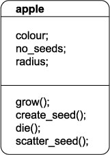
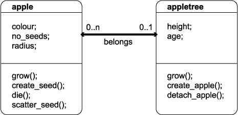
1.5.03. Simple UML relationship diagram

  • Classes
    • Attributes
    • Methods
  • Relationships
    • Participation
    • Cardinality
    • Roles

UML simple relationship diagram

1.5.04. UML inheritance

  • Notion of inheritance
    • Java parallel
    • 'is a' relationships
    • Database Student
      • is a Computer Science Student
        • is an Engineering Faculty Student
          • is a Student
            • is a Person
    • Inheritance hierarchies
  • UML diagrams can be used to show inheritance

UML class diagram, basic inheritance

1.5.05. UML diagram

  • Classes
  • Relationships
  • Inheritance

UML class diagram showing inheritance

2. DBMS Systems

This is the DBMS Systems course theme.
[Complete set of notes PDF 625Kb]

2.1. Queries

In this lecture we look at...
[Section notes PDF 319Kb]

2.1.01 Introduction

  • Methods of getting data out
  • The need for queries
  • QBE
  • SQL (design side)
    • History
    • Schemas and relations (CREATE)
    • Data types and domains
    • DROP and ALTER

2.1.02. Querying interfaces

  • High (view) level
  • Query-By-Example (QBE)
    • Alternative to SQL
      • Table driven (visually similar to relations)
      • Rather than script driven, hence intuitive over learned
      • Visual or text based
    • User fills in templates
    • Microsoft Access approach

    Query-by-example from MS Access

2.1.02b. QBE visual example

  • Record advancing
  • Query designing
    • Finite domain attributes
    • Web search parallel

Record manoeuvring in Visual QBE (Access)Query definition in Visual QBE (Access)

2.1.03. QBE text-format example

  • P. print, I. insert, D. delete, U. update
  • _VARNAME, copy field value into variable

Query by example (Text)

2.1.05. SQL

  • Structured Query Language
  • Success of relational databases
  • Developed for SystemR at IBM
  • ANSI standardised
  • SQL-1986 (SQL1), ongoing extension
  • SQL-1992 (SQL2), current version (Oracle 9i)
  • SQL-1999 (SQL3), regular expression matching, recursive queries
  • SQL-2003, XML features, auto-generated columns

2.1.05b. SQL command syntax

  • Where follows here is a brief summary
    • Oracle syntax
    • Similar but not identical to MySQL/MSSQL
  • General familiarity
  • Query writing best learnt by doing it
  • Lecture live-example
  • Coursework 1 will be SQL
  • Oracle (9i) SQL reference
  • MySQL (5.0) SQL reference

2.1.05c. SQL in application

  • Keyword oriented language
  • Keywords not congruous with Relational model
  • Lots of different ways to write SQL
    • Analogous to C/Java formatting
    • if (b==2) { a=1; } else { a=0; }
  • Recommend using case to differentiate attributes and keywords
    • SELECT colour, size, shape FROM fruit WHERE weight>22;
  • Oracle user accounts on Teaching database
  • Namespace references, e.g. shared.cars

2.1.06. SQL Create schema

  • Data definition commands
  • CREATE
    • SCHEMA <schema_name> AUTHORIZATION <a>
    • or workspace
  • Beware of names
    • Name collisions produce odd behaviours
  • SQL Schema embraces Tables (relations), constraints, views, domains, authorizations

2.1.07. SQL Create table

  • CREATE TABLE
    • <schema_name>.<relation_name>
    • (
      • <attribute_definitions>
      • <key>
      • <constraints>
    • )
  • CREATE TABLE example (Oracle)
  • Tables can (and should) be indexed by user
  • e.g. <username>.<tablename>
  • Normal login implies username
  • Non-local table access

2.1.08. Data types and domains (Oracle)

  • Numeric
    • ENUM
    • NUMBER, NUMBER(i), NUMBER(i,j)
      • Formatted numbers, i precision, j scale
      • (number of digits total, after decimal point)
    • Character-string
      • CHAR(n) - n is length
      • VARCHAR2(n) - n is max
    • DESCRIBE output example
    • Multi-database comparison of Datatypes
    • Database legacy: limited storage necessitated efficient storage
    • Does it need to be efficient anymore?

    You might consider all SQL types as being conceptually similar to attribute types in the relational model, although in reality the implementation of these types in a DBMS only approximates the mathematical purity of unordered domain sets etc.

2.1.08b. Data types and domains (MySQL)

  • Numeric
    • TINYINT, INT, INT UNSIGNED
    • FLOAT, DOUBLE, DECIMAL
    • ENUM
    • Character-string
      • CHAR(n) - n is length
      • VARCHAR(n) - n is max
      • TINYTEXT, TEXT
      • Beware different default/maximum lengths to Oracle
    • BLOB
    • Multi-database comparison of Datatypes

2.1.09. Time-based data types

  • Date and Time
    • DATE
      • Ten positions, components YYYY-MM-DD
    • TIME
      • Eight positions, components HH:MM:SS
    • TIME(i)
      • Time fractional seconds precision
      • Adds i+1 positions
    • TIMESTAMP
      • optionally WITH TIME ZONE
    • Very sensitive to syntactical ambiguities
      • day/month/year/hour/minute separators

2.1.10. DROPing

  • DROP <object> <obj_name> <flags>
  • DROP SCHEMA <schema_name> CASCADE
    • drops all workspace tables, domains
  • DROP TABLE <relation_name> RESTRICT
    • only drops table if
    • not referenced in any constraints/views
  • Notion of cascading
  • Table links

2.1.11. ALTERing

  • Schema evolution
  • Design side
  • ALTER TABLE <schema_name>.<relation_name> ADD
    <var_name> <var_type>;
  • Example
    • ALTER TABLE uni.student ADD hall VARCHAR(32);
  • Upper and lower case syntax
  • Naming conventions

2.1.12. Queries

  • Helper interfaces
    • HeidiSQL/phpMyAdmin/Sword/SQLplus
    • Design/perform a lot of routine queries for you
    • Important to learn SQL, reinforcement
    • Designing select queries is more difficult
    • Visual interfaces still lacking in this area
  • Select queries in SQL
  • Basic singlets
  • Renaming
  • Queries with Joins
  • Nested queries

2.1.13. SQL Queries

  • SELECT statement
  • Similar to relational data model SELECT then PROJECT
    • SELECT <attribute list>
    • FROM <table list>
    • WHERE <condition>;

Select query cropping example

2.1.14. SQL Queries

  • SELECT <attr_list>
    • FROM R,S,T
    • WHERE DNO = 10
  • equivalent to
  • p<attr_list>(sDNO=10 (R X S X T))
  • True-false evaluation tuple by tuple
  • WHERE clause as compound logical statement

2.1.15. SQL Queries

  • Produces a relation/set of tuples
  • Can be used to extract a single tuple
  • e.g. SELECT bday, age
    • FROM student
    • WHERE fname='Tim' AND lname='Smith'
    • Result = (13-05-80, 20)
  • Argument quoting (')
    • SQL poisoning
    • Not null
    • Not numeric values
  • MySQL Attribute quoting (`)
    • Hypothetical attribute `all`, all, and ALL

SQL poisoning is a vulnerability exposed by inadequate escaping of arguments/variables used to compose SQL queries.

E.g. Tim in previous example, could be Tim'; DELETE FROM student;' SELECT * FROM student WHERE 1

2.1.16. Renaming and referencing

  • AS keyword
  • (Partial) Attribute renaming in projection list
    • SELECT fname AS firstName, minit, lname AS surname...
  • Role names for relations
    • SELECT S.FNAME, F.FNAME, S.LNAME
      • FROM STUDENT AS S, STUDENT AS F
      • WHERE S.LNAME=F.LNAME
  • (Total) Attribute renaming in FROM
    • SELECT s.firstName, s.surname
      • FROM student AS s(firstName,surname,DOB,NINO,tutor)
  • Wildcards (SELECT s.* FROM...)

2.1.17. SQL Tables

  • Relations are bags, not sets
    • e.g. projection of non-key attributes
  • Set cannot contain duplicate item/repetition
  • Duplicates exist in bags and be:
    • SELECT DISTINCT (eliminated)
    • SELECT ALL (ignored/kept)


2.1.18. Queries and Joins

  • Relational database allows inter-related data
  • SQL select FROM gives Cartesian product
  • WHERE clause defines join condition
    • SELECT proj.pnum, mgr.ssn
    • FROM project AS proj, employee AS mgr
    • WHERE proj.mgrssn = mgr.ssn;
  • Alternatively, explicitly define join (note type)
    • SELECT project.pnum, employee.ssn
    • FROM project INNER JOIN employee
    • ON project.mgrssn = employee.ssn;

2.1.18b. Outer joins

  • Outer joins are crucial in the real-world
  • Databases often contain NULLs (3VL)
  • Analysis of where the crucial data is across a relationship
  • Previous example, only get project data for managed projects
    • SELECT project.*, employee.*
    • FROM project INNER JOIN employee
    • ON project.mgrssn = employee.ssn;

Inner join example

2.1.18c. Outer joins (cont)

  • Scale of loss isn't always instantly obvious
  • NULLs often used unpredicably
  • May want project information, even if no employee attached as manager
    • SELECT project.*, employee.*
    • FROM project LEFT OUTER JOIN employee
    • ON project.mgrssn = employee.ssn;

    Outer join example

    2.1.19. 2y and 3y joins

    • Queries can encapsulate any number of relations
      • Even one relation many times (in different roles)
    • Relationship chain
    • Across many relations
      • Tuples as Entities OR Relationships
    • e.g. Employee -> Works_on -> Project -> Department ->
      Manager

    2.1.20. Recursive closure

    • Can’t be done in SQL2
    • Recursive relationships
    • Unknown number of steps
    • SQL2 can’t generalise in single query

    2.1.21. Nested queries

    • Essential one or more (inner) queries within an (outer) query
    • Inner and outer query
    • Not to be confused with inner and outer joins
    • Inner query can go in three places
      • SELECT clause (projection list)
        • Must return a single value, then aliased as attribute in outer result
      • FROM clause
        • Inner query result used as standard table in FROM cross product
      • WHERE clause

    2.1.21b. Nested query example

    • Use of query result as comparator for other (outer) query
      • SELECT DISTINCT course
      • FROM dept WHERE course IN (
        • SELECT d.course
        • FROM dept AS d, faculty AS f, student AS s
        • WHERE d.ownfac=f.id AND s.owndept=d.id
        • AND f.name='Eng' AND s.year='3'
      • ) OR course IN (
        • SELECT course
        • FROM dept
        • WHERE code LIKE 'COMS3%');

    2.1.22. Bridging SQL across 3 tiers

    • Three tier database design
    • Changing role of DBMS
    • Indices
    • Aggregate functions (conceptual)
      • Over bags and sub-bags
    • Creating and updating views (ext)
    • SQL embedding

    Three tier database design (Internal, Conceptual, External)

    In this subsection we look at the different roles SQL play across the three tiers of database design. We discuss the areas in which SQL is lacking and how those difficiencies can be complemented by embedding SQL in other languages.

    2.1.25. Indices

    • Low/Internal level
    • Index by one attribute
    • For queries selecting by that attribute:
      • Faster tuple access (ordered tuples)
      • Reduces database memory load
        • Small cross product relation, only crosses requisites
      • Accelerates query resolution time
    • CREATE INDEX Index_Name ON RELATION(Attribute);

    2.1.26. Aggregate functions

    • Run over groups of tuples
    • Takes a projected attribute list as an argument
    • Produce relation with single tuple
    • SUM, MAX, MIN, AVG, COUNT
    • e.g. AggFunc over all tuples
      • SELECT SUM(SALARY), MAX(SALARY), MIN(SALARY)
      • FROM EMPLOYEE;
    • Single attribute lists (distinct values)
    • Multi-attribute lists (granularity of distinct values by pairing)

    2.1.27. Aggregates over sub-bags

    • Can run over subsets of tuples
    • GROUP BY keyword
    • Specifies the grouping attributes
    • Need to also appear in projected attr_list
    • Show result along side value for group attr
    • e.g. AggFunc over subgroups
      • SELECT dno, COUNT(*)
      • FROM employee
      • GROUP BY dno

    Quick SQL check, do all attributes in the SELECT projection list appear in the GROUP BY projection list.

    2.1.28. Creating views

    • Views are partial projections
    • Virtual relations, or views of live relations
    • Update synchronised
      • CREATE VIEW <virtual_relname>
      • AS <real_relation>
    • Real relation could be a query result
    • Clever bit is the change propagation
    • UPDATEs made to the view dataset are flooded back to relations
      • INSERT and DELETE behaviour needs to be defined
      • Non-trivial as INSERT into view (virtual relation) may leave holes in real relation

    2.1.29. Embedding SQL

    • SQL (alone) can do lots of clever things in one expression
    • But can only execute a single expression
    • Can structure SQL commands into proper programming languages
    • Java Database Connection (JDBC)
      • javac, then java VM
    • COBOL, C or PASCAL
      • precompiled with PRO*COBOL or PRO*C
    • Procedure Language (PL/SQL)
      • Oracle/MySQL procedural language
      • Stored procedures can take parameters

    2.2. Internals

    In this lecture we look at...
    [Section notes PDF 180Kb]

    2.2.01. Introduction

    • Database internals (base tier)
    • RAID technology
      • Reliability and performance improvement
    • Record and field basics
    • Headers to hashing
    • Index structures

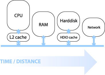
    2.2.01b. Machine architecture (by distance)

    • Distance from chip determines minimum latency
    • Speed of light is a constant
    • Impact of bus frequencies
      • IDE (66,100,133 Hz)
      • PCI, PCI-X (66,100,133 Hz)
      • PCI Express (1Ghz to 12Ghz)
    • Impact of bus bandwidths
      • PCI (32/64 bit/cycle, 133MB/s)
      • PCI Express (x16 8.0GB/s)

    Computer components by distance from processor

    Here's a link from Intel showing a machine architecture with signal bandwidths: Intel diagram

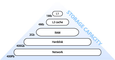
    2.2.01c. Machine architecture (by capacity)

    • Capacity increased with distance
    • Staged architecture as compromise
    • Speed, time/distance
    • Also cost, heat, usage scale

    Computer components by capacity

    2.2.02. Database internals

    • Stored as files of records (of data values)
      • Auxiliary data structures/indices
    • 1y and 2y storage
      • memory hierarchy (pyramid diagram)
      • volatility
    • Online and offline devices
    • Primary file organisation, records on disk
      • Heap - unordered
      • Sorted - ordered, sequential by sort key
      • Hashed - ordered by hash key
      • B-trees - more complex

    2.2.03. Disk fundamentals

    • DBMS task
      • linked to backup
    • 1y, 2y and 3y
      • e.g. DLT tape
    • Changing face of current technology
      • Impact of inexpensive harddisks
      • Flash memory devices (CF, USB)
    • Random versus sequential access
    • Latency (rotational delay) and
    • Bandwidth (data transfer rate)

    2.2.04. RAID technology

    • Redundant Array of Independent Disks
    • Data striping
      • Blocks (512 bytes), bits and transparency
    • Reliability (1/n)
      • Mirroring/shadowing
      • Error correction codes/parity
    • Performance (n)
      • Mirroring (2x read access)
      • Multiple parallel access

    2.2.05. RAID levels

    • 0 No redundant data
    • 1 Disk mirrors (performance gain)
    • 2 Hamming codes (also detect)
    • 3 Single parity disk
    • 4 Block level striping
    • 5 and parity/data distribution
    • 6 Reed-Soloman codes

    2.2.06. Records and fields

    • DBMS specific, generally
    • Records (tuples) comprise fields (attributes)
    • File is a sequence of records
    • Variable length records
      • Variable length fields
      • Multi-valued attributes/repeating fields
      • Optional fields
      • Mixed file of different record types

    2.2.07. Fields

    • records -> files -> disks
    • Fixed length for efficient access
    • Networking issues
    • Delimit variable length fields (max)
    • Explicit record/field lengths
    • Separators (,;,:,$,?,%)
    • Record headers and footers
    • Spanning
      • block boundaries and redundancy

    2.2.08. Primary organisation

    • Bias data manipulation to 1y memory
      • Load record to 1y, write back
      • Cache theorem
    • Data storage investment, rapidity of access
      • optimisations based on frequent algorithmic use
    • Ordering, ordering field/key field
    • Hashing

    2.2.09. Indexes/indices

    • Auxiliary structures/secondary access path
    • Single level indexes (Key, Pointer)
    • File of records
    • Ordering key field
    • Primary, Secondary and Clustering

    2.2.09b. Primary index example

    • Primary index on simple table
    • Ordering key field (primary key) is Integer
    • Pointers as addresses
    • Sparse, not dense

    Database example of primary key structure

    2.2.10. Primary Index file (as pairs list)

    • Two fields <K(i),P(i)>
    • Ordering key field and pointer to block
    • Second example, indexing candidate key Surname
      • K(1)="Barnes",P(1) -> block 1
        • Barnes record is first/anchor entry in block 1
      • K(2)="Smith",P(2) -> block 6
      • K(3)="Zeta",P(3) -> block 8
    • Dense (K(i) for every record), or Sparse
    • Enforce key constraint

    2.2.10b. Clustering index example

    • Clustering index
    • Ordering key field (OKF) is non-key
    • Each entry points to multiple records

    Database clustering index example

    2.2.11. Clustering Index (as pairs list)

    • Two fields <K(i),P(i)>
    • Ordering non-key field and pointer to block
      • Internal structure e.g. linked list of records
    • Each block may contain multiple records
      • K(1)="Barnes",P(1) -> block 1
      • K(2)="Bates",P(2) -> block 2
      • K(3)="Zeta",P(3) -> block 3
    • K(i) not required to have
      • a distinct value for each record
      • non-dense, sparse

    2.2.11b. Secondary Index example

    • Independent of primary ordering
    • Can't use block anchors
    • Needs to be dense

    Databases Secondary index example

    2.2.12. More indices

    • Single level index
      • ordered index file
      • limited by binary search
    • Multi level indices
      • based on tree data structures (B+/B-trees)
        • faster reduction of search space (logfobi)

    2.2.13. Indices

    • Database architecture
      • Intension/extension
    • Indexes separated from data file
      • Created/disgraded dynamically
      • Typically 2y to avoid reordering records on disk

    2.2.14. Query optimisation

    • Faster query resolution
      • improved performance
      • lower load
      • hardware cost:performance ratio
    • Moore's law
    • Query process chain
    • Query optimisation

    2.2.15. Query processing

    • Compile-track familiarity
      • Scanner/tokeniser - break into tokens
      • Parser - semantic understanding, grammar
      • Validated - check attribute names
        • Query tree
        • Execution strategy, heuristic
      • Query optimisation
        • In (extended relational) canonical algebra form

    2.2.16. Query optimisation

    • SQL query
      • SELECT lname, fname
      • FROM employee
      • WHERE salary > (
        • SELECT MAX(salary)
        • FROM employee
        • WHERE dno=5
      • );
    • Worst-case
      • Process inner for each outer
    • Best-base
    • Canonical algrebraic form

    2.2.16b. Query optimisation implementation

    • Indexing accelerates query resolution
    • Closed comparison (intra-tuple)
      • all variables/attributes within single tuple
      • e.g. x < 100
    • Open comparison (inter-tuple)
      • variables span multiple tuples
    • Essentially a sorting problem
    • Internal sorting covered (pre-requisites)
    • Need external sort for non-cached lists

    2.2.17. Query optimisation

    • External sorting
      • Stems from large disk (2y), small memory (1y)
      • Sort-merge strategy
        • Sort runs (small sets of total data file)
        • Then merge runs back together
      • Used in
        • SELECT, to accelerate selection (by index)
        • PROJECT, to eliminate duplicates
        • JOIN, UNION and INTERSECTION

    2.3. B-trees

    In this lecture we look at...
    [Section notes PDF 159Kb]

    2.3.01. Hash tables

    • Used to implement Indicies
    • O(n) access
    • Ordering Key Field (K) as argument to Hash function H()
    • Address H(K) maps to pointer

    Hash table example

    2.3.02. Tree structure

    • Tree revision
    • Node based
    • Branching nodes/leaf nodes
    • Parent/child nodes
    • Root node
    • Cardinality

    Basic tree structure

    2.3.03. Multi-level indices

    • Multi-level indices
    • One index indexes another
    • Implemented by multiple hash-tables
    • <H(k),P> pairs
    • (data far right)

    Multi-level indices by hash table

    2.3.04. Index zipping

    • Collapsing a single index
    • Two columns become one
    • <H(k),P> pairs sequentially stored
    • Common in the Elmasri

    Index zipping

    2.3.05. B-tree

    • Paritioning structure
    • Each node contains keys & pointers
    • Pointers can be:
      • Node pointers - to child nodes
      • Data pointers - to records in heap
    • Number of keys = Number of pointers - 1
    • Every node in the tree is identical

    B tree

    2.3.06. B+ trees

    • Similar to B-trees
    • Different types of nodes
      • Branching nodes
      • Leaf nodes
    • Each branching node has:
    • At most U children (max U)
    • At least L children (min L)
    • U = 2L, or U = 2L-1

    B+ tree

    2.3.07. Properties of B+ trees

    • Balanced
    • All leaf nodes at same level
    • Record search takes same time for every record
    • Partitioning needs to be comprehensive
    • B-tree: a1 < x < a2
    • B+tree: a1 <= x <= a2
    • Why?
      • because all data for partition values must be in the lowest level of the tree

    2.3.08. B+ tree operations

    • Insert operation cascades from bottom
    • Rules: node can contain U children (max)
    • Node combine
      • Legal if child nodes contain L children
      • Parent loses one key/paritition value
    • Node split
      • Legal if node contains U children
      • Parent node gains one key/partition value
        • Can cause cascade up tree & rebalancing

    B+ tree operations

    3. Database Design

    This is the Database Design course theme.
    [Complete set of notes PDF 300Kb].

    3.1. Functional Dependency

    In this lecture we look at...
    [Section notes PDF 48Kb]

    3.1.01. Introduction

    • What is relational design?
      • Notion of attribute distribution
      • Conceptual-level optimisation
    • How do we asses the quality of a design?

    3.1.02. Value in design

    • Allocated arbitrarily by DBD under ER/EER
    • Goodness at
      • Internal/storage level (base relations only)
        • Reducing nulls - obvious storage benefits /frequent
        • Reducing redundancy - for efficient storage/anomalies
      • Conceptual level
        • Semantics of the attributes /single entity:relation
        • No spurious tuple generation /no match Attr,-PK/FK

    3.1.03. Initial state

    • Database design
    • Universal relation
      • R = {A1, A2, …, An}
      • Set of functional dependencies F
    • Decompose R using F to
      • D = {R1, R2, …, Rn}
      • D is a decomposition of R under F

    3.1.05. Aims

    • Attribute preservation
      • Union of all decomposed relations = original
    • Lossless/non-additive join
      • For every extension, total join of r(Ri) yeilds r(R)
      • no spurious/erroneous tuples

    3.1.06. Aims (preservation)

    • Dependency preservation
      • Constraints on the database
        • X -> Y in F of R, appears directly in Ri
      • Attributes X and Y all contained in Ri
      • Each relation Ri in 3NF
    • But what's a dependency?

    3.1.07. Functional dependency

    • Constraint between two sets of attributes
      • Formal method for grouping attributes
    • DB as one single universal relation/-literal
      • R = {A1,A2,…,An}
      • Two sets of attributes, X subset R,Y subset R
    • Functional dependency (FD or f.d.) X -> Y
    • If t1[X] = t2[X], then t1[Y] = t2[Y]
      • Values of the Y attribute depend on value of X
      • X functionally determines Y, not reverse necessarily

    3.1.08. Dependency derivation

    • Rules of inference
    • reflexive: if X implies Y then X -> Y
    • augment: {X -> Y} then XZ -> YZ
    • transitive: {X -> Y,Y -> Z} then X -> Z
    • Armstrong demonstrated complete for closures

    3.1.09. Functional dependency

    • If X is a key (primary and/or candidate)
      • All tuples ti have a unique value for X
      • No two tuples (t1,t2) share a value of X
    • Therefore X -> Y
      • For any subset of attributes Y
    • Examples
      • SSN -> {Fname, Minit, Lname}
      • {Country of issue, Driving license no} -> SSN
      • Mobile area code -> Mobile
        network (not anymore)

    3.1.10. Process

    • Typically start with set of f.d., F
      • determined from semantics of attributes
    • Then use IR1,2,3 to infer additional f.d.s
    • Determine left hand sides (Xs)
      • Then determine all attributes dependent on X
    • For each set of attributes X,
      • determine X+ :the set of attributes f.d'ed by X on F

    3.1.11. Algorithm

    • Compute the closure of X under F: X+
      • xplus = x;
      • do
        • oldxplus = xplus;
        • for (each f.d. Y -> Z in F)
          • if (xplus implies Y) then
          • xplus = xplus union Z;
      • while (xplus != oldxplus);

    3.1.12. Function dependency

    • Consider a relation schema R(A,B,C,D) and a set F of functional dependencies
      • Aim to find all keys (minimal superkeys),
      • by determining closures of all possible X subsets of R’s attributes, e.g.
        • A+, B+, C+, D+,
        • AB+, AC+, AD+, BC+, BD+, CD+
        • ABC+, ABD+, BCD+
        • ABCD+

    3.1.13. Worked example

    • Let R be a relational schema R(A, B, C, D)
    • Simple set of f.d.s
    • AB -> C, C -> D, D -> A
    • Calculate singletons
      • A+, B+, C+, D+,
    • Pairs
      • AB+, AC+,…
    • Triples
      • and so on

    3.1.14. Worked example

    • Compute sets of closures
      • AB -> C, C -> D, D -> A
    • 1.Singletons
      • A+ -> A
      • B+ -> B
      • C+ -> CDA
      • D+ -> AD
    • Question: are any singletons superkeys?

    3.1.15. F.d. closure example

    • 2.Pairs (note commutative)
      • AB+ -> ABCD
      • AC+ -> ACD
      • AD+ -> AD
      • BC+ -> ABCD
      • BD+ -> ABCD
      • CD+ -> ACD
    • Superkeys?

    3.1.16. F.d. closure example

    • 3.Triples
      • ABC+ -> ABCD
      • ABD+ -> ABCD
      • BCD+ -> ABCD
    • Superkeys? Minimal superkeys (keys)?
    • 4.Quadruples
      • ABCD+ -> ABCD

    3.1.17. F.d. closure summary

    • Superkeys:
      • AB, BC, BD, ABC, ABD, BCD, ABCD
    • Minimal superkeys (keys)
      • AB, BC, BD

    3.2. Normal Forms

    In this lecture we look at...
    [Section notes PDF 121Kb]

    3.2.01. Orthogonal design

    • Information Principle:
      • The entire information content of the database is represented in one and only one way, namely as explicit values in column positions in tables
    • Implies that two relations cannot have the same meaning
      • unless they explicitly have the same design/attributes (including name)

    3.2.02. Normalization

    • Reduced redundancy
    • Organised data efficiently
    • Improves data consistency
      • Reduces chance of update anomalies
      • Data duplicated, then updated in only one location
    • Only duplicate primary key
      • All non-key data stored only once
    • Data spread across multiple tables, instead of one Universal relation R

    3.2.03. Good or bad?

    • Depends on Application
    • OLTP (Transaction processing)
      • Lots of small transactions
      • Need to execute updates quickly
    • OLAP (Analytical processing/DSS)
      • Largely Read-only
      • Redundant data copies facilitate Business Intellegence applications, e.g. star schema (later)
    • 3NF considered ‘normalised’
      • save special cases

    3.2.04. Normal forms (1NF)

    • First Normal form (1NF)
      • Disallows multivalued attributes
      • Part of the basic relational model
    • Domain must include only atomic values
      • simple, indivisible
    • Value of attribute-tuple in extension of schema
    • t[Ai] ∈ (Ai)

    3.2.05. Normalisation (1NF)

    • Remove fields containing comma separated lists
    • Multi-valued attribute (AMV) of Ri
    • Create new relation (RNEW)
      • with FK to Ri[PK]
      • RNEW(UID, AMV, FKI)

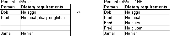
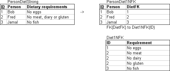
    3.2.06. Normalisation (1NF)

    • On weak entity
    • On strong entity

    weak entity example
    strong entity example

    3.2.07. Normal forms (2NF)

    • A relation Ri is in 2NF if:
      • Every nonprime attribute A in Ri is
      • fully functionally dependent on 1y key of R
    • If all keys are singletons, guaranteed
    • If Ri has composite key are
      • all non-key attributes fully functionally dependent
      • on all attributes of composite key?

    3.2.08. Normal forms (2NF)

    • Second normal form (2NF)
      • Full functional dependency X → Y
        • A ∈ X, (X - {A}) ¬→ Y
    • If any attribute A is removed from X
    • Then X → Y no longer holds
      • Partial functional dependency
      • A ∈ X, (X - {A}) → Y

    3.2.09. Normal forms (2NF)

    • In context
      • Not 2NF: AB → C, A → C
        • AB → C is not in 2NF, because B can be removed
      • Not 2NF: AB → CDE, B → DE
        • because attributes D&E are dependent on part of the composite key (B of AB), not all of it

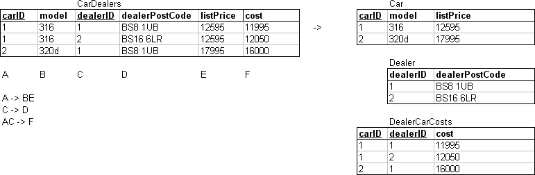
    3.2.10. Normalisation (2NF)

    • Split attributes not depended on all of the primary key into separate relations

    3.2.11. Normal forms (BCNF)

    • Boyce-Codd Normal form (BCNF)
      • Simpler, stricter 3NF
        • BCNF → 3NF
        • 3NF does not imply BCNF
      • nontrivial functional dependency X → Y
      • Then X must be a superkey

    3.2.12. Normal forms (3NF)

    • Third Normal form (3NF)
    • Derived/based on transitive dependency
    • For all nontrivial functional dependencies
      X → A
    • Either X must be a superkey
    • Or A is a prime attribute
      (member of a key)

    3.2.13. Normal forms in context

    • AB → C, C → D, D → A
    • In context
      • 3NF? Yes
        • Because AB is a superkey and
        • D and A are prime attributes
      • BCNF? No
        • Because C and D are not superkeys
        • (even though AB is)

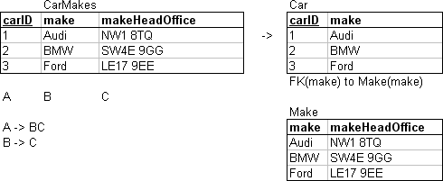
    3.2.14. Normalisation (3NF)

    • CarMakes not in 3NF because:
      • singleton key A
      • non-trivial fd B → C
        • B not superkey, C not prime attribute


    3.3. OODB

    In this lecture we look at...
    [Section notes PDF 34Kb]

    3.3.01. Introduction

    • Database architectures, beyond
    • Why OODBMS?
    • ObjectStore
    • CORBA object distribution standard

    3.3.02. Large DBMS

    • Complex entity fragmentation
      • across many relations
    • Breaks the miniworld-realworld dichotomy
    • Requires conceptual abstracting layer
    • Difficult to retrieve all information for x
    • Compounded by version control

    3.3.03. Object orientation

    • Object components (icv triples)
      • Object Identity (OID), I
        • replaces primary key
      • Type constructor, c
        • how the object state is constructed from sub-comp
        • e.g. atom, tuple (struct), set, list, bag, array
      • Object state, v
      • Object behaviour/action

    3.3.04. Desirable features

    • Encapsulation
      • Abstract data types
      • Information hiding
    • Object classes and behavior
      • Defined by operations (methods)
    • Inheritance and hierarchies
    • Strong typing (no illegal casting)
      • don’t think about inheritance just yet

    3.3.05. Desirable features

    • Persistence
      • Objects exist after termination
      • Naming and reachability mechanism
      • Late binding in Java
    • Performance
      • user-def functions executed on server, not client
    • Extension into relational model
      • Domains of objects, not just values
      • Domain hierarchies etc.

    3.3.06. Desirable features

    • Polymorphism
      • aka. operator overloading
      • same method name/symbol
      • multiple implementations
    • Easy link to Programming languages
      • popular OO language like Java/C++
      • Better than PL/SQL integration
      • Much better than PL-JDBC integration!
    • Highly suitable for multimedia data

    3.3.07. Undesirable features

    • Object Ids
      • Artificial Real-Mini, double edged sword
      • Exposes inner workings (suspended abstraction)
    • Lack of integrity constraints
    • No concept of normalisation/forms
    • Extreme encapsulation
      • e.g. creation of many accessor/mutator methods
    • Lack of (better) standardisation

    3.3.08. More undesirables

    • Originally no mechanism for specifying
    • relationships between objects
    • In RDBMS – relationships are tuples
    • In OODBMS – relationships should be properties of objects

    3.3.09. ObjectStore

    • Packages supporting Java or C++
    • C++ package uses:
      • C++ class definition for DDL
      • insert(e), remove(e) and create collections, for DML
    • Bidirectional relationship facility
    • Persistency transparency
      • Identical pointers to persistent and transient objects

    3.3.10. CORBA

    • Common Object Request Broker Architecture
    • Object communication (unifying paradigm)
      • Distributed
      • Heterogeneous
      • Network, OS and language transparency
    • Java implementation org.omg.CORBA
    • Also C, C++, ADA, SMALLTALK

    3.4. Type Inheritance and EER diagrams

    In this lecture we look at...
    [Section notes PDF 117Kb]

    3.4.01. Introduction

    • Design/schema side (Entity types)
    • Object-orientated concepts
      • Java, C++ or UML
      • Sub/superclasses and inheritance
    • EER diagrams
    • EER to Relational mapping

    3.4.02. OO

    • Inheritance concept
      • Attributes (and methods)
    • Subtypes and supertypes
    • Specialisation and Generalisation
    • ER diagrams
      • show entities/entity sets
    • EER diagrams
      • show type inheritance
      • additional 8th step to ER→Relational mapping

    3.4.03. Objects

    • Basic guide to Java
    • Object, classes as blueprints
    • Object, collection of methods and attributes
    • Miniworld model of real world things
    • Object, entity in database terms

    3.4.04. Abstract

    • Similar objects
    • Car Park example
    • Student example
    • Shared properties/attributes
    • Generalisation
    • Reverse, specialisation

    3.4.05. Relationships

    • Using English as model
    • ‘Is a’ (inheritance)
    • ‘Has a’ (containment)
    • Nouns as objects
    • Verbs as methods
    • Adjectives as variables (sort of)

    3.4.06. Classes

    • Superclasses (Student)
    • Subclasses (Engineer, Geographer, Medic)
    • Inheritance
    • Subclass inherits superclass attributes
      • Union of specific/local and general attributes
    • Inheritance chains
      • Person → Student → Engineer → Computer Scientist

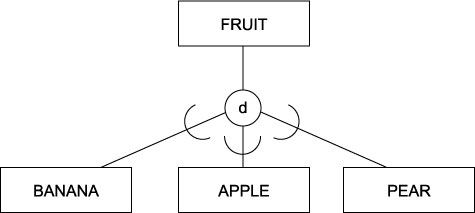
    3.4.07. EER Fruit example

    • Partial participation
    • Disjoint subclasses
    • A fruit may be either a pear or an apple or a banana, or none of them. A fruit may not be a pear and a banana, an apple and a banana, an apple and a pear …

    Extended Entity-Relationship diagram showing partial participation in disjoint subclasses

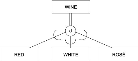
    3.4.08. EER Wine example

    • Total, disjoint
    • Equivalent to Java Abstract classes
    • A Wine has to be either Red, White or Rosé cannot be both more

    EER diagram showing total participation in disjoint subclasses

    3.4.09. More extended (EER)

    • Specialisation lattices
      • and Hierarchies
    • Multiple inheritance
    • Union of two superclasses (u in circle)
    • In addition to basic ER notation

    3.4.10. EER diagramatic notation

    • Subset symbol to illustrate
    • sub/superclass relationship
    • direction of relationship
    • Circle to link super to subclasses
      • Disjoint
      • Overlapping
      • Union

    3.4.11. Disjointness constraint

    • Disjointness (d in circle) – single honours
    • Overlapping (o in circle) – joint honours/sports
    • Membership condition on same attribute
      • attribute-defined specialisation
      • defining attribute
      • implies disjointness
    • versus user-defined
      • each entity type specifically defined by user

    3.4.12. Completeness constraint

    • Total specialisation
      • Every entity in the superclass must be a member of atleast 1 subclass
      • Double line (as ER)
    • Partial specialisation
      • Some entites may belong to atleast 1 subclass, or none at all
      • Single line
    • Yields 4 possibilities
      • (Total-Dis, Total-Over, Partial-Dis, Partial-Over)

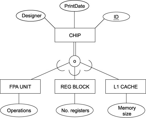
    3.4.13. EER Chip example

    • Total, overlapping
    • A Chip may has to be at least one of FPA Unit, Reg Block, L1 Cache, and may be more than one type

    EER diagram showing total participation in overlapping sets

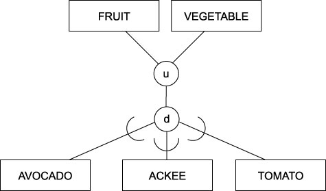
    3.4.14. EER Multiple inheritance

    • Type hierarchies
    • Specialisation lattices
    • Well, sir, the Supreme Court of the United States has determined that the tomato is for legal and commercial purposes both a fruit and a vegetable. So we can legally refer to tomato juice as 'vegetable' juice.
    • Candice, General Foods

    EER diagram showing Multiple inheritance

    3.4.15. EER to Relational Mapping

    • Initially following 7 ER stages
    • Stage 8
    • 4 different options
      • Optimal solution based on problem
    • Let C be superclass, S1..m subclasses

    3.4.16. Stage 8

    • Create relation for C, and relations for S1..m each with a foreign key to C (primary key)
    • Create relations for S1..m each including all attributes of C and its primary key

    3.4.17. Stage 8

    • Create a single relation including all attributes of C ∪ S1..m and a type/discriminating attribute
      • only for disjoint subclasses
    • Create a single relation as above, but include a boolean type flag for each subclass
      • works for overlapping, and also disjoint

    3.5. System Design

    In this lecture we look at...
    [Section notes PDF 64Kb]

    3.5.01. Databases in Application

    • Where’s the data?
    • Programmer driven future
    • OODBMS limitations
    • RDBMS longevity
    • System design by
      • Data store, delivery, interface
    • Case study

    3.5.02. Where’s the data?

    • Previously covered distance from User to Data (and reason for it)
    • Client-Server data model creates DBMS
      • P2P alternative
    • Accountability
    • Distribution (BitTorrent, eDonkey)
    • Caching

    3.5.03. Where’s the data?

    • Answer: everywhere
    • But where is it meaningful?
    • Answer: for whom?

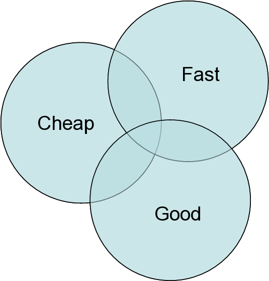
    3.5.04. Quality paradigm

    • Large projects require large teams
    • Team overhead (ref 2nd year)
    • Code responsibilities
    • Data/data model resp.
    • Object responsibilities

    3.5.05. Web application data support

    • Web application programming
    • Goal, dynamically produced XHTML
    • Client side designer-programmer split
      • CSS, XHTML
    • Server side programmer-programmer split
      • Old school: query design, integrator
      • New school: MVC (Model-View-Controller)
        • Controller – user input
        • Model – modelling of external world
        • View – visual feedback

    3.5.06. CMS

    • Content Management System
    • part of other courses
    • CMS is a DBMS
    • Zope/Plone and ZODB
    • e107, Drupal and Seagull
    • Zend MVC Framework (pre-beta)

    3.5.07. OODBMS limitations

    • Future unknown
    • RDBMS supports
      • Application data sharing
      • Physical/logical data independence/views
      • Concurrency control
      • Constraints
    • at inception these requirements not known
    • RDBMS mathematical basis → extensible
    • Crude Type Inheritance (see EER mapping)
    • OODBMS as construction kit

    3.5.08. Weaknesses in RDBMS

    • Data type support
    • Unwieldy, created 3VL (nulls)
    • Type Inheritance and Relationships
    • Tuple:Entity fragmentation
      • not to be confused with ‘fragmentation’
    • Entity approximation requires joins

    3.5.09. System design

    • Client specifications
    • Variance amongst Mobile devices
    • Rich-media Content delivery
    • Where’s the data? (M – media database)
    • Where’s it going? (C – mobile browser)
    • How’s it going to get there? (query design)
    • What’s it going to look like? (V – XHTML)

    3.5.10. Muddy boots

    • The real world of databases
    • Massive Excel spreadsheets
    • Access Migration
    • Normalisation
    • Update implications
    • Visual language of the Internet limitations
    • Future of browser components

    3.6. Design for optimised query resolution

    • Skillswap talk
    • 28th May 2008

    3.6.01. Introduction

    • Pace of talk
    • Principals not query syntax
    • Online notes
    • Questions welcome anytime
    • Prompt thought about the issues

    3.6.02. Terms

    3.6.03. Domains and sets

    • Domains
      • Set of possible data
      • 8-bit unsigned integer example
    • Powersets
      • Set
        • Odd numbers less than 10
        • (1,3,5,7,9)
      • Powerset
        • Set of sets
          • 5 digit collection of non-repeating integers less than 10
          • ((1,3,5,7,9),(2,3,5,7,9),(1,4,5,7,9),(1,3,6,7,9)...)

    3.6.04. Query and snapshot

    • Query + database snapshot returns one set of actual data
      • but a query alone defines a powerset of possible data
    • Load
      • Metrics for query performance
      • Time is easy to measure
      • Load is better in the real world
        • Query might be fast to execute, but require a lot of memory

    3.6.05. Design in context

    • Query design needs context
      • Hardware information
      • Competition information (other Application Servers)
        • MySQL, Apache, Tomcat, SVN
      • Data information
        • Likely number of rows, lifetime of information, interval distribution within domains
      • Database design information
      • Database implementation information
        • Transaction granularity
      • Use information
        • Balance between read (SELECT) and write (INSERT, UPDATE, DELETE) ops

    3.6.06. Elementary steps

    • Ask MySQL what it's doing
      • Query analysis with EXPLAIN
    • Cache the query
      • no free lunch, there's almost always a cost
      • Simple
        • Repetitive queries
        • Rare since requires constant snapshot
        • What's the point of the query

    3.6.07. Query caching

    • Complex - Summary table
      • Multiple queries drawing data from subset of DB data
      • Cache subset
        • Query subset rather than whole database
    • Complex - Age analyses
      • Webstats, meaningful even if not last 24 hours
        • Run the heavyweight analysis queries during downtime
        • Cache results

    3.6.08. Avoid the query

    • Cache the object
      • Higher level primitives
      • Object persistence
    • Get only the critical data
      • What's critical now
      • What's required in 10s, 1m, 5m

    3.6.09. Simplify

    • Route/path to information
      • Introduction
        • Join is an arc, join time is arc length
        • Table is a node
      • Graph traversal problem
        • Dijkstra's shortest path
          • Heuristic
            • Search for optimal
            • General, each node defines a population of tuples

    3.6.10. Traversal

    • Traversal of graph
      • (aka. positive closure)
      • gives intermediate relation
    • Goal
      • Intermediate relation minimisation
        • Space (memory, disk triangle)
        • Time (fast joins versus slow joins)
          • Fewer relations
          • Fewer active attributes (horizontal cropping)
          • Fewer rows (vertical cropping)
            • Role of single-relation WHERE statements

    3.6.11. Optimise (Indexing)

    • Giving the Optimiser hints
    • Indexing
      • Simple - single attribute
        • Index(A)
        • Reduce sparse domains (e.g. text)
      • Composite - multiple attributes (typically pairs)
        • Index (A,B)
        • Some subtleties in here

    3.6.12. Optimise (Limit)

    • Limit
      • Valueable on sorts (0,10 faster than 0,1000!)
      • Beware limit referencing
        • Limit 1000,10 will fetch the first 1000, then give you the 10 you want
          • Search engines
        • Better to use WHERE restriction if possible

    3.6.13. Optimise (Delayed Joins)

    • SELECT FROM (SELECT id FROM ... LIMIT 0,10)
      • Subqueries not the silver bullet
      • Often not cached or indexed
    • Views help manage complex relationships but not performance
    • Changing picture
      • Even between MySQL 5.0 and 5.1
      • MySQL 6.0
        • Falcon (transactional) Storage
        • Better subquery optimisation

    3.6.14. References

    4. Distributed systems

    This is the Distributed systems course theme.

    [Complete set of notes PDF 109Kb]

    4.1. Transaction processing

    In this lecture we look at...
    [Section notes PDF 86Kb]

    4.1.01. Distributed Databases

    • Transactions
    • Unpredictable failure
      • Commit and rollback
    • Stored procedures
    • Brief PL overview
      • Cursors

    4.1.02. Transactions

    • Real world database actions
    • Rarely single step
    • Flight reservation example
      • Add passenger details to roster
      • Charge passenger credit card
      • Update seats available
      • Order extra vegetarian meal

    4.1.04. Desirable properties of transactions

    ACID test

    • Atomicity
      • transaction as smallest unit of processing
      • transactions complete entirely or not at all
        • consequences of partial completion in flight example
    • Consistency
      • complete execution preserves database constrained state/integrity
      • e.g. Should a transaction create an entity with a foreign key then the reference entity must exist (see 4 constraints)

    4.1.05. ACID test continued

    • Isolation
      • not interfered with by any other concurrent transactions
    • Durable (permanency)
      • commited changes persist in the database, not vulernable to failure

    4.1.06. Commit

    • Notion of Commit (durability)
    • Transaction failures
      • From flight reservation example
        • Add passenger details to roster
        • Charge passenger credit card
        • Update seats available: No seats remaining
        • Order extra vegetarian meal
    • Rollback

    4.1.07. PL/SQL overview

    • Language format
      • Declarations
      • Execution
      • Exceptions
      • Handling I/O
      • Functions
      • Cursors

    4.1.08. PL/SQL

    • Blocks broken into three parts
      • Declaration
        • Variables declared and initialised
      • Execution
        • Variables manipulated/actioned
      • Exception
        • Error raised and handled during exec

    • DECLARE
          ---declarations
      BEGIN
          ---statements
      EXCEPTION
          ---handlers
      END ;

    4.1.09. Declaration

    • DECLARE
      • age NUMBER;
      • name VARCHAR(20);
      • surname employee.fname%TYPE;
      • addr student.termAddress%TYPE;

    4.1.10. Execution

    • BEGIN (not in order)
      • /* sql_statements */
        • UPDATE employee SET salary = salary+1;
      • /* conditionals */
        • IF (age < 0) THEN
          • age: = 0;
        • ELSE
          • age: = age + 1;
        • END IF;
      • /* transaction processing */
        • COMMIT; ROLLBACK;
      • /* loops */ /* cursors */
    • [END;] (if no exception handling)

    4.1.11. Exception passing

    • Beginnings of PL I/O
    • CREATE TABLE temp (logmessage varchar(80));
      • Can create transfer/bridge relation outside

    • Within block (e.g. within exception handler)
      • WHEN invalid_age THEN
        • INSERT INTO temp VALUES( ‘Cannot have negative ages’);
      • END;

      • SELECT * FROM temp;
        • To review error messages

    4.1.12. Exception handling

    • DECLARE
      • invalid_age exception;
    • BEGIN
      • IF (age < 0) THEN
        • RAISE invalid_age
      • END IF;
    • EXCEPTION
      • WHEN invalid_age THEN
        • INSERT INTO temp VALUES( ‘Cannot have negative ages’);
      • END;

    4.1.13. Cursors

    • Cursors
      • Tuple by tuple processing of relations
      • Three phases (two)
        • Declare
        • Use
        • Exception (as per normal raise)

    4.1.14. Impact

    • PL blocks coherently change database state
    • No runtime I/O
    • Difficult to debug
    • SQL tested independently

    4.1.15. PL Cursors

    • DECLARE
    • name_attr EMPLOYEE.NAME%TYPE;
    • ssn_attr EMPLOYEE.SSN%TYPE;
    • /* cursor declaration */
    • CURSOR myEmployeeCursor IS
      • SELECT NAME,SSN FROM EMPLOYEE
      • WHERE DNO=1
      • FOR UPDATE;
    • emp_tuple myEmployeeCursor%ROWTYPE;

    4.1.16. Cursors execution

    • BEGIN
    • /* open cursor */
    • OPEN myEmployeeCursor;
    • /* can pull a tuple attributes into variables */
    • FETCH myEmployeeCursor INTO name_attr,ssn_attr;
    • /* or pull tuple into tuple variable */
    • FETCH myEmployeeCursor INTO emp_tuple;
    • CLOSE myEmployeeCursor;


    • [LOOP…END LOOP example on handout]

    4.1.17. Concurrency Introduction

    • Concurrent transactions
    • Distributed databases (DDB)
    • Fragmentation
    • Desirable transaction properties
    • Concurrency control techniques
      • Locking
      • Timestamps

    4.1.18. Notation

    • Language
      • PL too complex/long-winded
    • Simplified database model
      • Database as collection of named items
      • Granularity, or size of data item
      • Disk block based, each block X
    • Basic transaction language (BTL)
      • read_item(X);
      • write_item(X);
      • Basic algebra, X=X+N;

    4.1.19. Transaction processing

    • DBMS Multiuser system
      • Multiple terminals/clients
        • Single processor, client side execution
      • Single centralised database
        • Multiprocessor, server
        • Resolving many transactions simultaneously
    • Concurrency issue
      • Coverage by previous courses (e.g. COMS12100)
      • PL/SQL scripts (Transactions) as processes
    • Interleaved execution

    4.1.20. Transactions

    • Two transactions, T1 and T2
    • Overlapping read-sets and write-sets
    • Interleaved execution
    • Concurrency control required
    • PL/SQL example
      • Commit; and rollback;

    4.1.21. Concurrency issues

    • Three potential problems
      • Lost update
      • Dirty read
      • Incorrect summary
    • All exemplified using BTL
      • Transaction diagrams to make clearer
      • C-like syntax for familiarity
      • Many possible examples of each problem

    4.1.22. Lost update

    • T1
    • read_item(X);
    • X=X-N;

    • write_item(X);
    • read_item(Y);

    • Y=Y+N;
    • write_item(Y);
    • T2

    • read_item(X);
    • X=X+M;

    • write_item(X);
    • T1 X update overwritten

    4.1.23. Dirty read (or Temporary update)

    • T1
    • read_item(X);
    • X=X-N;
    • write_item(X);

    • <T1 fails>
    • <T1 rollback>

    • read_item(X);
    • X=X+N;
    • write_item(X);
    • T2

    • read_item(X);
    • X=X+M;
    • write_item(X);
    • T2 reads temporary incorrect value of X

    4.1.24. Incorrect summary

    • T1

    • read_item(X);
    • X=X-N;
    • write_item(X);

    • read_item(Y);
    • Y=Y-N;
    • write_item(Y);
    • T2
    • sum=0;
    • read_item(A)
    • sum=sum+A;

    • read_item(X);
    • sum=sum+X;
    • read_item(Y);
    • sum=sum+Y;
    • T2 sums after X-N and before Y-N

    4.1.25. Serializability

    • Schedule S is a collection of transactions (Ti)
    • Serial schedule S1
      • Transactions executed one after the other
      • Performed in a serial order
      • No interleaving
      • Commit or abort of active transaction (Ti) triggers
        execution of the next (Ti+1)
      • If transactions are independent
        • all serial schedules are correct

    4.1.26. Serializability

    • Serial schedules/histories
      • No concurrency
      • Unfair timeslicing
    • Non-serial schedule S2 of n transactions
      • Serializable if
    • equivalent to some serial schedule of the same n transactions
      • correct
    • n! serial schedules, more non-serial

    4.1.27. Distribution

    • DDB, collection of
      • multiple logically interrelated databases
      • distributed over a computer network
      • DDBMS
    • Multiprocessor environments
      • Shared memory
      • Shared disk
      • Shared nothing

    4.1.28. Advantages

    • Distribution transparency
      • Multiple transparency levels
      • Network
      • Location/dept autonomy
      • Naming
      • Replication
      • Fragmentation
    • Reliability and availability
    • Performance, data localisation
    • Expansion

    4.1.29. Fragmentation

    • Breaking the database into
      • logical units
      • for distribution (DDB design)
    • Global directory to keep track/abstract
    • Fragmentation schema/allocation schema
      • Relational
      • Horizontal
        • Derived (referential), complete (by union)
      • Vertical
      • Hybrid

    4.1.30. Concurrency control in DDBs

    • Multiple copies
    • Failure of individual sites (hosts/servers)
    • Failure of network/links
    • Transaction processing
      • Distributed commit
      • Deadlock
    • Primary/coordinator site - voting

    4.1.31. Distributed commit

    • Coordinator elected
    • Coordinator prepares
      • writes log to disk, open sockets, sends out queries
    • Process
      • Coordinator sends ‘Ready-commit’ message
      • Peers send back ‘Ready-OK’
      • Coordinator sends ‘Commit’ message
      • Peers send back ‘Commit-OK’ message

    4.1.32. Query processing

    • Data transfer costs of query processing
      • Local bias
      • High remote access cost
      • Vast data quantities to build intermediate relations
    • Decomposition
      • Subqueries resolved locally

    4.1.33. Concurrency control

    • Must avoid 3+ problems
      • Lost update, dirty read, incorrect summary
      • Deadlock/livelock - dining example
    • Data item granularity
    • Solutions
      • Protocols, validation
      • Locking
      • Timestamps

    4.1.34. Definition of terms

    • Binary (two-state) locks
    • locked, unlocked associated with item X
    • Mutual exclusion
    • Four requirements
      • Must lock before access
      • Must unlock after all access
      • No relocking of already locked
      • No unlocking of already unlocked

    4.1.35. Definition

    • Multiple mode locking
    • Read/write locks
    • aka. shared/exclusive locks
    • Less restrictive (CREW)
    • read_lock(X), write_lock(X), unlock(X)
      • e.g. acquire read/write_lock
      • not reading or writing the lock state


    4.1.36. Rules of Multimode locks

    • Must hold read/write_lock to read
    • Must hold write_lock to write
    • Must unlock after all access
    • Cannot upgrade/downgrade locks
      • Cannot request new lock while holding one
    • Upgrading permissable (read lock to write)
      • if currently holding sole read access
    • Downgrading permissable (write lock to read)
      • if currently holding write lock

    4.2. Concurrency protocols

    In this lecture we look at...
    [Section notes PDF 37Kb]

    4.2.01. Introduction

    • Concurrency control protocols
    • Concurrency techniques
      • Locks, Protocols, Timestamps
      • Multimode locking with conversion
    • Guarenteeing serializability
    • Associated cost
    • Timestamps and ordering

    4.2.02. Guarenteeing serializability

    • Two phase locking protocol (2PL)
      • Growing/expanding
        • Acquisition of all locks
        • Or upgrading of existing locks
      • Shrinking
        • Release of locks
        • Or downgrading
      • Guarentees serializability
        • equivalency without checking schedules

    4.2.03. A typical transaction pair

    • T1

    • read_lock(Y);
    • read_item(Y);
    • unlock(Y);

    • write_lock(X);
    • read_item(X);
    • X=X+Y;
    • write_item(X);
    • unlock(X);
    • T2

    • read_lock(X);
    • read_item(X);
    • unlock(X);

    • write_lock(Y);
    • read_item(Y);
    • Y=X+Y;
    • write_item(Y);
    • unlock(Y);
    • Violates rules of two phase locking
    • unlock occurs during locking/expanding phase

    4.2.04. 2PL: Guaranteed serializable

    • T1

    • read_lock(Y);
    • read_item(Y);
    • write_lock(X);
    • unlock(Y);
    • read_item(X);
    • X=X+Y;
    • write_item(X);
    • unlock(X);
    • T2

    • read_lock(X);
    • read_item(X);
    • write_lock(Y);
    • unlock(X);
    • read_item(Y);
    • Y=X+Y;
    • write_item(Y);
    • unlock(Y);
    • Less efficient (cost), but serializable

    4.2.05. Guarantee cost

    • T2 ends up waiting for read access to X
    • Either after T1 finished
      • T1 cannot release X even though it has finished using it
      • Incorrect phase (still expanding)
    • Or before T1 has used it
      • T1 has to claim X during expansion, even if it doesn’t use
        it until later
    • Cost: limits the amount of concurrency

    4.2.06. Alternatives

    • Concurrency control
      • Locks limit concurrency
        • Busy waiting
      • Timestamp ordering (TO)
      • Order transaction execution
        • for a particular equivalent serial schedule
        • of transactions ordered by timestamp value
          • Note: difference to lock serial equivalent
      • No locks, no deadlock

    4.2.07. Timestamps

    • Unique identifier for transaction (T)
    • Assigned in order of submission
      • Time
        • linear time, current date/sys clock - one per cycle
      • Counter
        • counter, finite bitspace, wrap-around issues
      • Timestamp aka. Transaction start time
      • TS(T)

    4.2.08. Timestamping

    • DBMS associates two TS with each item


    • Read_TS(X): gets read timestamp of item X
      • timestamp of most recent successful read on X
      • = TS(T) where T is youngest read transaction


    • Write_TS(X): gets write timestamp of item X
      • as for read timestamp

    4.2.09. Timestamping

    • Transaction T issues read_item(X)
      • TO algorithm compares TS(T) with Write_TS(X)
      • Ensures transaction order execution not violated
    • If successful,Write_TS(X) <= TS(T)
      • Read_TS(X) = MAXTS(T), current Read_TS(X)
    • If fail,Write_TS(X) > TS(T)
      • T aborted, rolled-back and resubmitted with new TS
      • Cascading rollback

    4.2.10. Timestamping

    • Transaction T issues write_item(X)
      • TO algorithm compares TS(T) with Read_TS(X) and compares TS(T) with Write_TS(X)
    • If successful, op_TS(X) <= TS(T)
      • Write_TS(X) = TS(T)
    • If fail, op_TS(X) > TS(T)
      • T aborted, cascade etc.
    • All operations focus on not violating the execution order defined by the timestamp ordering

    4.2.11. Updates

    • Insertion
      • 2PL: DBMS secures exclusive write-lock
      • TOA: op_TS(X) set to TS(creating transaction)
    • Deletion
      • 2PL: as insert
      • TOA: waits to ensure later transactions don’t access
    • Phantom problem
      • Record being inserted matches inclusion conditions
      • of another transaction
        (e.g. selection by dno=5)
      • Locking doesn’t guarantee inclusion

        (need index locking)

    5. Real world

    This is the Real world course theme.

    [Complete set of notes PDF 206Kb]

    5.1. Web

    In this lecture we look at...
    [Section notes PDF 133Kb]

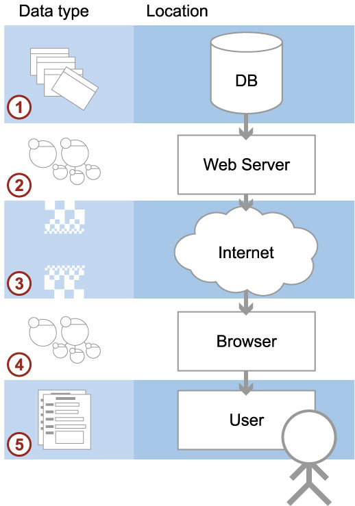
    5.1.01. Databases for the Internet

    • Path from DB to User
    • Information flow
    • Data formats (OO)
    • Format transitions
    • Limitations/channel
    • The Future

    5.1.02. OO

    • Object orientated approach
      • Consistent/optimised development model
      • Good approximation of real world
      • Closer link to mini-world
    • Java and PHP
    • DB persistence
    • UML

    5.1.03. Java and PHP in context

    • Java
      • JSP (server-side)
      • Javascript (client-side)
    • PHP
      • Server side only
    • JSON or XML
      • Object communication
    • Ideal scenario
      • Java – load times

    5.1.04. In a perfect world

    • Homogenous data format/data model
    • DB stores objects instead
    • Objects transferred
      • Robust
      • Lightweight
      • Fast
      • Consistent (more later in Transactions)
      • Caching

    5.1.05. In the real world

    • Heterogenous data model
    • Object translation/wrappers
    • Different languages features at different layers
    • Minimal subset of OO functionality available end-to-end
    • Going to look at information flow/functionality provided

    5.1.06. User

    • Limitations of being human
      • short term memory
      • long term familiarity
    • language of the Internet
      • hypertext linking
      • form filling
    • Advantages of being human
      • impatience, no waiting
      • wants instant response

    5.1.07. Browser

    • Http requests
    • Forms
      • Post
      • Get
    • Form fields
      • By name, by ID
      • Hidden
    • Javascript/DOM tree

    5.1.08. Internet

    • Communication medium
    • Good for transferring data
    • Not good for transforming data
    • e.g. Light in air
    • e.g. Signal over CAT5e/UTP cable

    5.1.09. Web server

    • Straight HTML pages
    • Dynamic HTML pages
      • PHP example
      • JSP example
    • As above with RDBMS integration
      • PHP PDO example
    • As above with Objects
      • PHP DBDO example

    5.1.10. load, edit, submit, act timeline

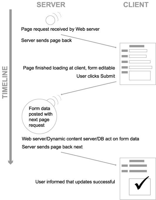
    5.1.11. href click, versus form post

    • Protocol stack
    • Basic up-down
    • Shortcuts
    • Browser cache
    • Web server
      • assembled page cache
      • php object cache
    • DB optimised queries

    5.1.12. Examples from the web

    5.2. Decision Support

    In this lecture we look at...
    [Section notes PDF 85Kb]

    5.2.01. Introduction

    • Decision support systems (DSS)
    • Duplicates of live systems, historical archiving
    • Primarily read-only
    • Load and refresh operations
    • Integrity
      • Assumptions about initial data
    • Large, indexed, redundancy

    5.2.02. DSS Management

    • Design
      • Logical
        • Temporal keys, required to distinquish historical data (since:to
          current & during:within interval)
      • Physical (Hash indexes, Bitmap indexes)
        • Controlled Redundancy
      • Synchronisation/update propogation
        • Synchronous (update driven)
        • Asynchronous (query driven)

    5.2.03. Data Preparation

    • Extract
      • pulling from live database system(s)
    • Cleansing
    • Transformation and Consolidation
      • migrating from live or legacy system design

        to DSS design
    • Load (DSS live/query-able)
    • Refresh (latest update)

    5.2.04. Querying

    • Boolean expression complexity
      • heavy WHERE clauses
    • Join complexity
      • Normalised databases, many tables
      • Facts distributed across tables
      • Joins required to answer complex questions
    • Function and Analytic complexity
      • Often require non-DBMS functions
      • Smaller queries with interleaved code


    5.2.05. Data Warehouse

    • Specific example of DSS
    • Subject-orientated
      • e.g. customers/products
    • Non-volatile
      • once inserted, items cannot be updated
    • Time variant
      • Temporal keys
    • Accuracy and granularity issues

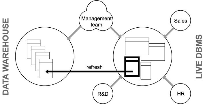
    5.2.06. DB Company organisation

    • By example

    5.2.07. Dimensional Schema

    • Consider product, customer, sales data
    • Each sale represents a specific event
      • when a product was purchased
      • when a customer bought something
      • when a sale was recorded
    • Each can be thought of as an axis

      or dimension (3D)
    • Each occurred at a moment in time (4D)

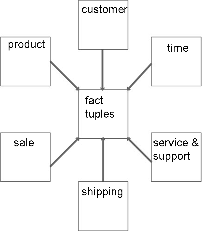
    5.2.08. Star schemae and Hypercubes

    • Data centralised in ‘fact’ table
    • Referencing creates star pattern
    • Dimensions as satellite tables
    • Normalising creates snowflake schema
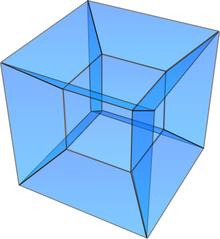
    5.2.09. Hypercubes

    • Hypercube is also a multi-processor topology inspired by a 4D shape
    • Used by Intel’s iPSC/2
    • Good at certain database operations
    • e.g. Duplicate removal
    • MIMD